GPU Programming, Part 1: Architecture, SIMT, Tensor Cores, Occupancy, and Precision

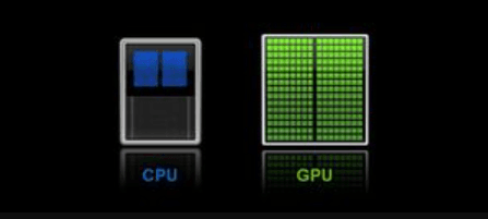
A modern server CPU and a datacenter GPU are both made of transistors on similar process nodes, but they spend those transistors on opposite goals.

• CPU is a latency machine: it is built to finish a single stream of instructions as quickly as possible.
• GPU is a throughput machine: it is built to finish an enormous number of identical operations per unit time, and it does not care how long any single one takes.

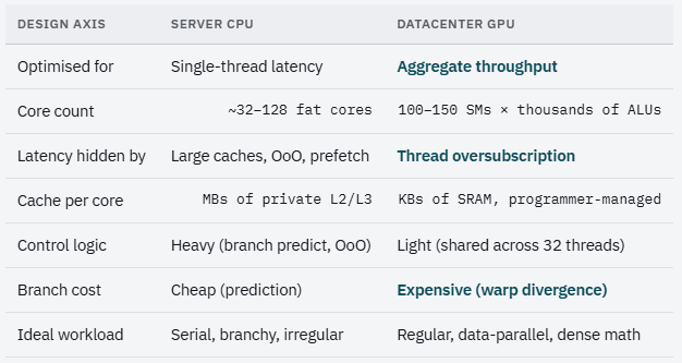
That difference cascades into the whole chip.

This is the first part of a GPU programming series. It focuses on building the mental models required to understand modern GPU systems: compute, memory hierarchies, collective communication, distributed training, orchestration, and inference. With that foundation established, later parts move beyond conceptual explanations into real implementations, writing kernels, analyzing performance, and reconstructing the core algorithms that power modern GPU software stacks. The goal is not to memorize CUDA APIs, but to develop an intuition for how GPU hardware executes code and why high-performance kernels are designed the way they are.

A CPU core devotes most of its area to making one thread fast: deep out-of-order pipelines, branch predictors, speculative execution, and above all large caches (tens of megabytes of L3) to keep that thread fed without waiting on DRAM.

A GPU inverts the ratio. It spends its area on arithmetic units, packs thousands of them onto the die, and accepts that any individual operation will stall waiting on memory.

It hides that stall not with a cache but with sheer parallelism: when one group of threads stalls on a memory load, the hardware instantly switches to another group that is ready to run.

For context, an NVIDIA H100 (SXM5) has 132 streaming multiprocessors, each capable of holding up to 64 warps (2,048 threads) resident simultaneously. That is over 250,000 threads in flight on one GPU, while a high-end server CPU runs perhaps 128–256 hardware threads total.

Let's have a look at what we discussed so far:

This also has a precise quantitative form. Little's Law, from queueing theory, relates the number of items simultaneously in a system to the rate they flow through and how long each stays:

L = λW

Concurrency L (items in flight) equals arrival/throughput rate λ times residence time W. To sustain a throughput λ when each operation takes W to complete, you must keep L = λW operations in flight at all times.

Say you are running a web server that handles requests, where each request takes 200 ms (0.2 seconds), and you want to process 500 requests per second. Using Little's Law:

• L = 500 × 0.2 = 100

This means your server must have 100 requests in progress simultaneously. If it only processes 20 requests at a time, it cannot reach 500 requests/second because each request stays busy for 0.2 seconds.

Now let's apply this to memory. To saturate HBM bandwidth, the number of bytes in flight must equal the bandwidth–latency product. This is the memory-system form of Little's Law, and it dictates the minimum parallelism (the memory-level parallelism) your kernel needs.

Bytes in flight needed to saturate H100 HBM:

1. Take HBM bandwidth λ = 3.35 × 10¹² B/s (H100 HBM3 peak) and memory latency W ≈ 400 cycles, a representative global-memory latency.
2. Convert latency to seconds at a ~1.5 GHz memory clock: W ≈ 400 / (1.5 × 10⁹) ≈ 2.67 × 10⁻⁷ s ≈ 267 ns. The clock is approximate; the point is the order of magnitude.
3. Bytes in flight: L = λW = 3.35 × 10¹² × 2.67 × 10⁻⁷ ≈ 8.9 × 10⁵ bytes ≈ 890 KB must be in the pipe simultaneously to hide the latency.
4. At 128 bytes per coalesced warp transaction, that is 8.9 × 10⁵ / 128 ≈ 6,900 outstanding warp-loads, out of a hardware maximum of 132 × 64 = 8,448 resident warps. You must keep the GPU ~80% full of memory-issuing warps just to saturate HBM, which is precisely why high occupancy matters for memory-bound kernels.

We said more warps hide more latency, and Little's Law makes it falsifiable: if your kernel keeps fewer than ~7,000 memory operations in flight, it cannot reach peak HBM bandwidth no matter how fast the memory is.

This is also why latency-bound kernels with low occupancy leave bandwidth on the table: they violate L = λW.

SIMT: how a GPU actually executes

NVIDIA calls its model SIMT (Single Instruction, Multiple Thread). It is a cousin of the SIMD (vector) model in CPUs, but with a crucial software-facing difference: you write code as if each thread is independent and scalar, and the hardware groups threads together and executes them in lockstep behind the scenes.

The unit of lockstep execution is the warp: exactly 32 threads on every NVIDIA GPU to date. All 32 threads in a warp share one program counter and issue the same instruction in the same cycle, each operating on its own data in its own registers.

The warp is the true atom of scheduling. The hardware never schedules a single thread, only warps. Threads are organized in a strict hierarchy, and every level maps to a physical resource.

• Thread: the scalar unit you write code for; has its own registers and program-counter state; maps to a lane in a warp.
• Warp: 32 threads executed in lockstep, the unit the SM schedulers actually dispatch. This is not exposed in source, but it governs performance.
• Thread block (CTA): up to 1,024 threads; resides entirely on one SM, shares that SM's fast shared memory, and can synchronize with __syncthreads().
• Thread-block cluster: Hopper/Blackwell only; a group of blocks on neighbouring SMs that can address each other's shared memory (distributed shared memory).
• Grid: all the blocks launched by one kernel, spread across every SM on the GPU.

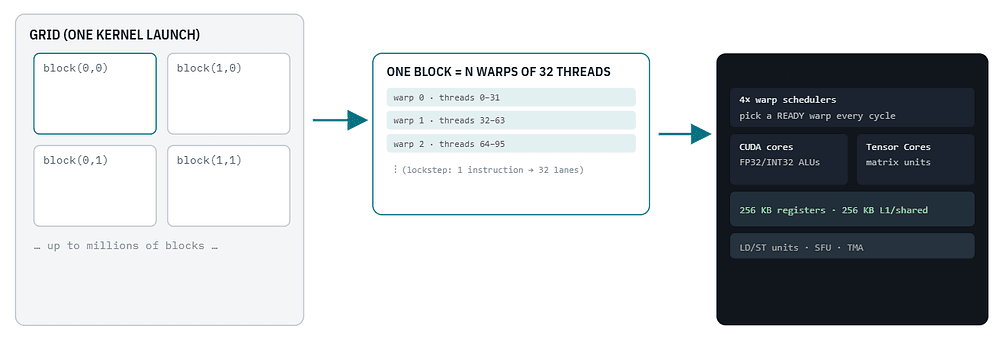
Your kernel launches a grid of blocks. Each block is assigned whole to one SM, where it is sliced into warps of 32 threads. The SM's warp schedulers keep many warps resident and switch between them every cycle to hide memory latency. This is throughput computing in one picture.

This is also where I want to discuss the Amdahl and Gustafson laws, which explain the limits of parallel speedup. Whenever you add GPUs (or SMs, or cores), these laws bound what you get.

Let p be the fraction of work that is parallelizable and N the number of workers. Then Amdahl's Law (fixed problem size):

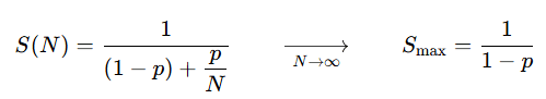
The brutal consequence is that even a 5% serial fraction (p = 0.95) caps speedup at 1 / 0.05 = 20x, no matter how many GPUs you buy.

This is the mathematical reason communication and synchronization overheads (the serial parts of distributed training) are so damaging, and it motivates everything about collectives and distributed training that we will get to later.

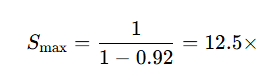
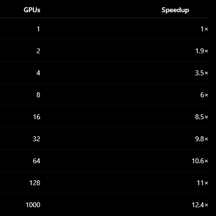
Suppose 8% of each training step is effectively serial (gradient all-reduce that doesn't overlap, optimizer step, data stalls), so p = 0.92. The maximum conceivable speedup from scaling out is:

At N = 64 GPUs you would get:

S(64) = 1 / (0.08 + 0.92 / 64) ≈ 10.6x

A scaling efficiency of 10.6 / 64 ≈ 17%. This is the answer to "why not buy more GPUs?"

So the important point is that shrinking the serial fraction (overlap, bigger batches to amortize comms) matters far more than adding nodes once you are deep into the Amdahl regime. Otherwise you will eventually be paying for hundreds of GPUs that barely improve performance.

Amdahl assumes a fixed problem: "I have one fixed training job. Can more GPUs finish it faster?" In practice we scale the problem with the machine (bigger models, bigger batches), which is the regime Gustafson's Law describes:

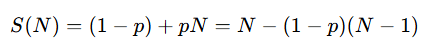
It asks "If I buy more GPUs, why not train a bigger model or larger batch?" Instead of making the same work smaller, you make the workload larger. Here speedup grows (nearly) linearly in N because the parallel work expands to fill the larger machine, which is why the formula becomes S(N) = (1 − p) + pN.

Since the parallel work grows with the machine, the speedup is almost linear. For p = 0.92 and N = 64:

S = 0.08 + 0.92 × 64 = 58.96

That is much closer to the ideal 64x than the 10.6x predicted by Amdahl. This is why weak scaling (more GPUs for a proportionally bigger job) looks so much healthier than strong scaling (more GPUs for the same job), and why training clusters are sold on the former.

Inside the streaming multiprocessor

The streaming multiprocessor (SM) is the GPU's fundamental compute building block, the rough analogue of a CPU core, except that one SM runs thousands of threads. For example, H100 has 132 of them and A100 has 108. Scaling a GPU up across generations is largely a matter of adding SMs and feeding them more memory bandwidth.

Each SM contains:

• A set of CUDA cores (the scalar FP32/INT32 ALUs).
• One or more Tensor Cores (matrix-multiply-accumulate units, the workhorses for deep learning).
• Load/store units.
• Special-function units (SFUs, for transcendentals like exp and sin).
• A large register file (256 KB on H100).
• A block of on-chip SRAM split between L1 cache and programmer-managed shared memory (256 KB combined on H100).
• A small number of warp schedulers (four on recent architectures).

The warp schedulers are where latency hiding happens. Each scheduler tracks a pool of resident warps, and every cycle it looks for a warp whose next instruction's operands are ready (not waiting on a pending memory load) and dispatches it.

If a warp issues a load from HBM (hundreds of cycles of latency), the scheduler simply sets it aside and issues from a different ready warp. As long as there are enough resident warps to cover the latency, the arithmetic units never go idle. This is why more threads is the GPU answer to hiding more latency.

Tensor Cores and the Transformer Engine

The plain CUDA cores do scalar FP32/INT math. The reason a GPU can train a transformer is the Tensor Core: a dedicated unit that performs a small matrix multiply-accumulate (e.g. a 4×4×4 or larger tile) in a single operation, at far higher throughput than issuing the equivalent scalar multiplies.

Because virtually all the FLOPs in a neural network are matrix multiplications (the linear layers, the attention projections), Tensor Cores deliver the order-of-magnitude speedups that make large-model training feasible.

Tensor Cores have evolved each generation in the precision they support:

• Volta introduced them at FP16.
• Ampere added TF32 and BF16.
• Hopper added FP8 with its Transformer Engine, a combination of FP8-capable Tensor Cores and runtime logic that automatically chooses FP8 vs 16-bit per layer and manages the scaling factors needed to keep FP8 numerically stable.
• Blackwell adds FP4 and FP6 and a second-generation Transformer Engine.

Warps in practice: divergence and your first kernel

Because a warp shares one program counter, a data-dependent branch where some of the 32 threads go one way and some go the other forces the hardware to execute both paths serially, masking off the inactive threads on each pass.

This is warp divergence, and it is one of the most common reasons a GPU kernel underperforms. A branch on threadIdx.x % 2 can halve your throughput, while a branch that is uniform across the warp costs nothing.

// Each thread computes one element of C = A + B.
// This is the canonical data-parallel pattern: no branches, no divergence.
__global__ void vecAdd(const float* A, const float* B, float* C, int n) {
  // Global thread index = which block + which lane within the block.
  int i = blockIdx.x * blockDim.x + threadIdx.x;
  if (i < n)                 // <-- uniform-ish guard; only the tail warp diverges
      C[i] = A[i] + B[i];    // one fused-ish op per thread, fully parallel
}

// GOOD: branch is uniform across the warp (all 32 threads take the same side),
// because warpId is constant for every lane in the warp.
__global__ void good_branch(const float* x, float* y, int n) {
  int i      = blockIdx.x * blockDim.x + threadIdx.x;
  int warpId = i / 32;                       // same value for all 32 lanes
  if (warpId % 2 == 0) y[i] = x[i] * 2.0f;   // entire warp goes one way -> no divergence
  else                 y[i] = x[i] * 3.0f;
}

// BAD: branch splits within the warp on the low bit of the lane id.
// The hardware executes BOTH sides serially with half the lanes masked: ~2x cost.
__global__ void bad_branch(const float* x, float* y, int n) {
  int i = blockIdx.x * blockDim.x + threadIdx.x;
  if (threadIdx.x % 2 == 0) y[i] = x[i] * 2.0f;   // lanes 0,2,4,...  active
  else                      y[i] = x[i] * 3.0f;   // lanes 1,3,5,...  active (serialised!)
}

Launching the kernel from the host:

int main() {
  int n = 1 << 24;                 // 16M elements
  size_t bytes = n * sizeof(float);
  float *dA, *dB, *dC;
  cudaMalloc(&dA, bytes); cudaMalloc(&dB, bytes); cudaMalloc(&dC, bytes);
  // ... copy inputs H2D with cudaMemcpy ...

  int threads = 256;                              // block size (multiple of 32!)
  int blocks  = (n + threads - 1) / threads;      // enough blocks to cover n
  vecAdd<<<blocks, threads>>>(dA, dB, dC, n);     // triple-angle = grid, block launch
  cudaDeviceSynchronize();                        // wait for the GPU

  cudaFree(dA); cudaFree(dB); cudaFree(dC);
}

Occupancy: the throughput budget

Occupancy is the ratio of warps actually resident on an SM to the hardware maximum (64 warps on recent architectures). It determines how much latency the schedulers can hide, since more resident warps means more ready work to switch to when others stall.

But occupancy is bounded by three finite per-SM resources, and a kernel hits the limit on whichever runs out first:

1. Registers per thread: the SM has a fixed register file (65,536 32-bit registers on recent GPUs). If each thread needs 64 registers, the SM can host 65,536 / 64 ≈ 1,024 threads = 32 warps = 50% occupancy, regardless of anything else.
2. Shared memory per block: if each block claims 48 KB of the 256 KB SRAM, at most ~5 blocks fit, capping resident threads.
3. Block / warp slots: hardware limits on blocks-per-SM and warps-per-SM.

Formally, the resident warps per SM is the minimum over three integer-floored constraints, and occupancy is that divided by the hardware maximum:

And here is how we define achieved occupancy:

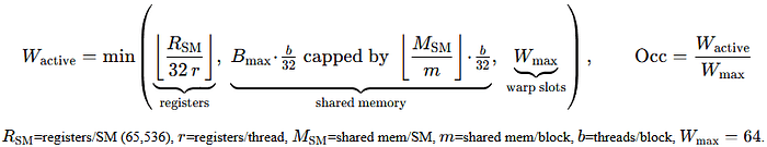
So for a kernel that uses r = 64 registers per thread on an SM with 65,536 registers:

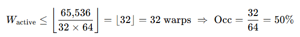
Even though the hardware supports 64 warps, we only have enough registers for 32 warps, which makes occupancy 50%. If you push register use down to r = 32, the ceiling doubles to 64 warps, and occupancy becomes 100%. But if each thread uses r = 128 (often what happens when the compiler runs out), you get 16 warps: 25% occupancy.

This is called the register cliff:

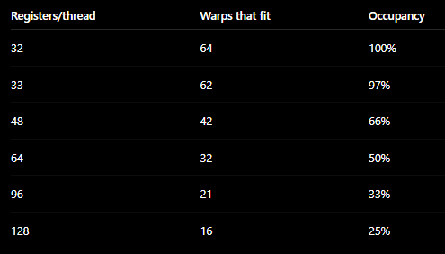
Occupancy is a step function of register pressure: small changes cross integer thresholds and produce sudden cliffs, which is why the occupancy calculator exists. You can do a similar exercise to see how differing shared-memory requirements from blocks change occupancy.

What is important here is that maximizing active warps is not the same as maximizing throughput. A kernel that uses more registers per thread to keep data in fast registers (doing more work per thread, a technique called register blocking) can beat a high-occupancy kernel that spills to memory. A register-blocked kernel deliberately raises the register count (lowering occupancy) to keep more operands in registers and do more work per thread.

The right objective is throughput = (work per thread) × (active warps) × (issue rate), and the maximum often sits below 100% occupancy, the classic result that 50–60% occupancy can beat 100%.

A failure mode worth naming is register spilling: when a kernel needs more registers than the SM can give at the desired occupancy, the compiler spills excess values to local memory (which lives in slow HBM, cached in L1), quietly destroying performance. NVIDIA's occupancy calculator and the --ptxas-options=-v compiler flag (which prints register and shared-memory usage) are the tools to reach for when tuning this.

Here is how to query occupancy at runtime:

// The CUDA runtime can tell you the best block size for max occupancy of a kernel.
int minGridSize, blockSize;
cudaOccupancyMaxPotentialBlockSize(&minGridSize, &blockSize,
                                 vecAdd, /*dynamicSMem=*/0, /*blockLimit=*/0);
// And how many blocks of a given size will be resident per SM:
int maxActiveBlocks;
cudaOccupancyMaxActiveBlocksPerMultiprocessor(&maxActiveBlocks, vecAdd, blockSize, 0);
// occupancy = (maxActiveBlocks * blockSize / 32) / maxWarpsPerSM

Numerical precision: the formats that define modern training

Half the art of large-model performance is using the lowest precision that still converges. Lower precision means fewer bytes moved, more values per Tensor Core operation, and more model in the same HBM.

Let's have a look at the numeric formats common to deep learning:

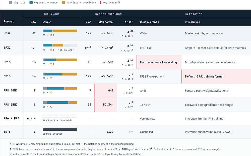
The two distinctions that matter most in conversation:

• FP16 vs BF16: they are the same size, but FP16 spends more bits on the mantissa (precision) and fewer on the exponent (range), while BF16 keeps FP32's full 8-bit exponent and sacrifices mantissa. In training, range matters more than precision: gradients span many orders of magnitude, and FP16's narrow exponent causes small gradients to underflow to zero, which is why FP16 training needs loss scaling (multiply the loss by a large constant before backprop to push gradients into the representable range, then unscale). BF16 has the same range as FP32, so it usually needs no loss scaling and has become the default.
• FP8's two flavors: Hopper's FP8 comes in two layouts because the forward and backward passes have different needs. E4M3 (4 exponent, 3 mantissa, range ±448) is used in the forward pass where precision helps, and E5M2 (5 exponent, 2 mantissa, range ±57,344) is used for gradients in the backward pass where range matters. Because FP8's range is tiny, values are kept in range with per-tensor scaling factors tracked by the Transformer Engine (it keeps a short history of the maximum absolute value, the amax, and rescales). FP8 typically buys ~30–40% throughput and ~2x memory over BF16, but is prone to divergence when activations have outliers beyond the range; the practical mitigation is finer-grained (per-block or per-token) scaling.

So when you ask "can I just train in FP8 and halve my GPU bill?", the credible answer is nuanced. FP8 gives real throughput and memory wins on Hopper/Blackwell, and the Transformer Engine automates most of the scaling, but it isn't free. Numerically sensitive layers (often the final projection, normalization, and sometimes attention) frequently stay in BF16, and you validate convergence on your own data before committing. The pattern that works is FP8 for the bulk of the matmuls with mixed-precision fallback, not FP8 everywhere.

The datacenter GPU lineage

Finally, it is good to know which hardware generation introduced what, along with memory capacity, bandwidth, and relative compute. The progression tells a story: each generation adds memory bandwidth and a lower-precision format, because both directly attack the bottlenecks of ever-larger models.

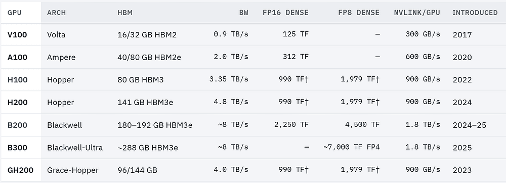
These are non-sparse (dense) rates; NVIDIA also quotes 2x sparse numbers that apply only with 2:4 structured sparsity. You should treat all vendor TFLOPS as best-case. There are three machines worth understanding as systems here.

H200 is an H100 with more memory. Same GH100 compute die, same TFLOPS; the only change is 141 GB of HBM3e at 4.8 TB/s versus 80 GB at 3.35 TB/s. So H200 helps exactly when you are memory-capacity or memory-bandwidth bound (models that don't fit in 80 GB, long context, large-batch memory-bound inference) and does nothing for compute-bound work.

GH200 Grace Hopper fuses one Grace ARM CPU (72 cores) with one Hopper GPU over NVLink-C2C at 900 GB/s, cache-coherent, roughly 7x the bandwidth of PCIe Gen5. This is important for workloads that spill to CPU memory or stream huge datasets, because the CPU's memory becomes almost a slow extension of GPU memory rather than a distant pool behind a thin PCIe straw.

GB200 NVL72 is the one to understand as an architectural shift. It is a liquid-cooled rack that wires 72 Blackwell GPUs and 36 Grace CPUs into a single NVLink domain via nine NVSwitch trays, giving ~130 TB/s of all-to-all bandwidth across the whole rack and presenting 13.5 TB of unified HBM3e. Inside that rack, the usual two-tier hierarchy (fast NVLink within a server, slower InfiniBand between servers) collapses. Tensor parallelism, which we will see is the most communication-hungry form of parallelism and normally must stay inside one 8-GPU server, can now span 72 GPUs over NVLink. That changes how you map a model onto the hardware, and we will cover it in a following part of the series.