GPU Architecture and Programming
Volume I, The Machine builds the modern GPU platform from first principles: the SIMT core, the memory hierarchy, the fabric that joins thousands of accelerators, distributed training, storage, scheduling, inference, operations, and the economics of the clouds that sell it. Each chapter is also paired with the mathematics that makes its claims precise. Volume II, The Kernel then descends into a single naive CUDA matrix multiply and reads every line at four altitudes: source code, user space, kernel space, and silicon, ending with the optimization ladder from coalescing to Tensor Cores.
Volume I · The Machine
GPU Architecture & the SIMT Execution Model
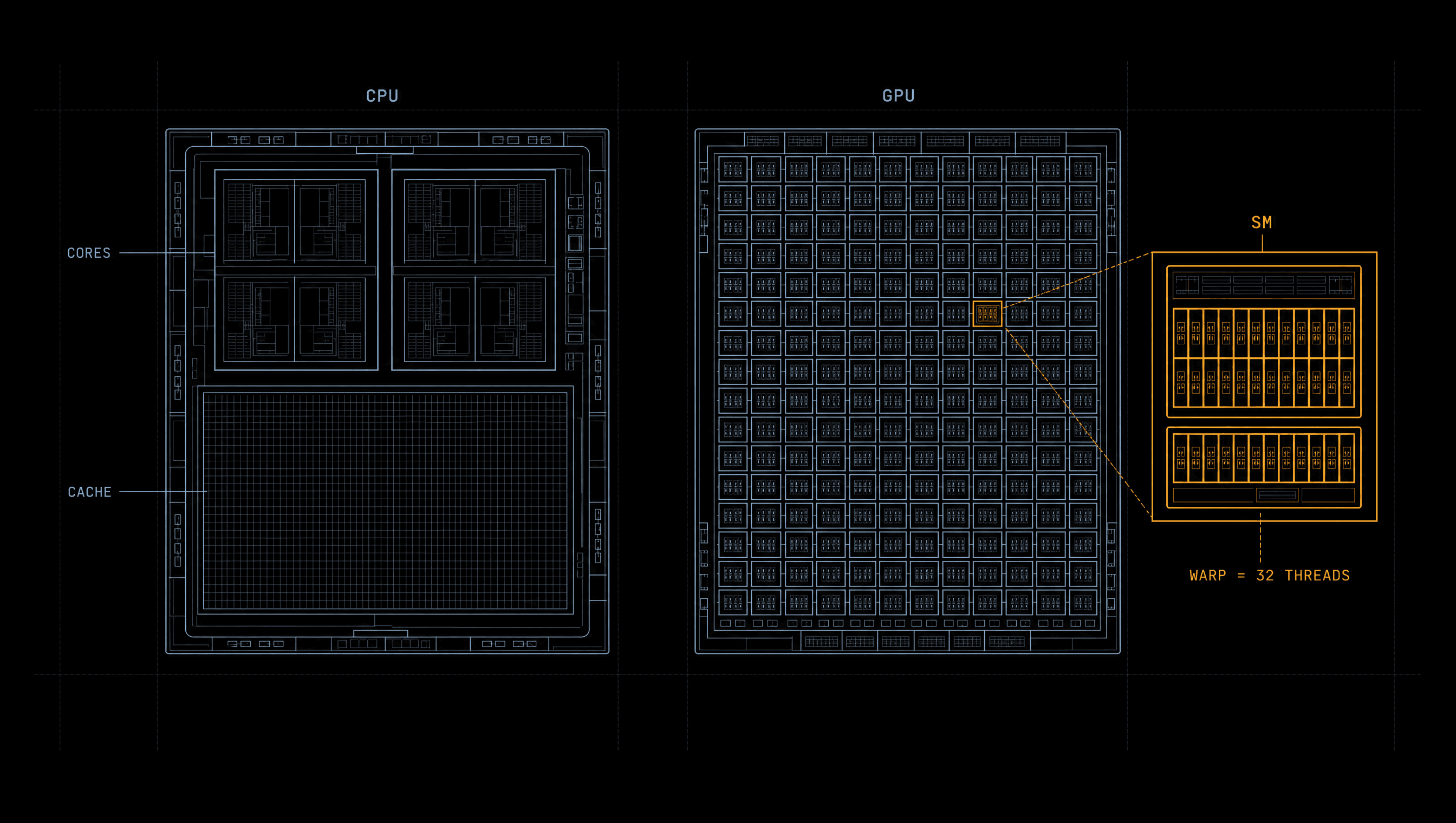
Before you can size a cluster or debug a 40%-utilization training run, you have to know what a single GPU actually is. GPU is a fundamentally different machine than CPU that trades latency for throughput. This chapter builds that machine from the transistor up.
Anyone building serious systems on GPUs is expected to move from “how many H100s does this need” all the way down to “why is this kernel only hitting 30% of peak FLOPS”, and back up to the business case, without losing the thread.
Two philosophies of silicon
A CPU minimizes the latency of one instruction stream, GPU maximizes the throughput of millions.
A modern server CPU and a datacenter GPU are both made of transistors on similar process nodes, but they spend those transistors on opposite goals. The CPU is a latency machine: it is built to finish a single stream of instructions as quickly as possible. The GPU is a throughput machine: it is built to finish an enormous number of identical operations per unit time, and it does not care how long any single one takes.
That difference cascades into the whole chip. A CPU core devotes most of its area to making one thread fast: deep out-of-order pipelines, branch predictors, speculative execution, and, above all, large caches (tens of megabytes of L3) to keep that thread fed without waiting on DRAM. A GPU inverts the ratio. It spends its area on arithmetic units, packs thousands of them onto the die, and accepts that any individual operation will stall waiting on memory. It hides that stall not with a cache but with sheer parallelism: when one group of threads stalls on a memory load, the hardware instantly switches to another group that is ready to run.
This is the single most important idea in the chapter, and the dividing line between people who have read about GPUs and people who understand them.
Table 1.1 shows where the transistors go on each side of the divide:
| Design axis | Server CPU | Datacenter GPU |
|---|---|---|
| Optimised for | Single-thread latency | Aggregate throughput |
| Core count | ~32–128 fat cores | 100–224 SMs × thousands of ALUs |
| Latency hidden by | Large caches, OoO, prefetch | Thread oversubscription |
| Cache per core | MBs of private L2/L3 | KBs of SRAM, programmer-managed |
| Control logic | Heavy (branch predict, OoO) | Light (shared across 32 threads) |
| Branch cost | Cheap (prediction) | Expensive (warp divergence) |
| Ideal workload | Serial, branchy, irregular | Regular, data-parallel, dense math |
SIMT: how a GPU executes
One instruction, 32 lanes: the warp is the atom of GPU scheduling.
NVIDIA calls its model SIMT, Single Instruction, Multiple Thread. It is a cousin of the SIMD (vector) model in CPUs, but with a crucial software-facing difference: you write code as if each thread is independent and scalar, and the hardware groups threads together and executes them in lockstep behind the scenes.
The unit of lockstep execution is the warp: exactly 32 threads on every NVIDIA GPU to date. All 32 threads in a warp share one program counter and issue the same instruction in the same cycle, each operating on its own data in its own registers. The warp is the true atom of scheduling, the hardware never schedules a single thread, only warps.
Threads are organised in a strict hierarchy, and every level maps to a physical resource.
Internalise this, because the entire CUDA programming model in Chapter 3 is built on it:
| Level | What it is, and what it maps to |
|---|---|
| Thread | The scalar unit you write code for. Has its own registers and program-counter state. Maps to a lane in a warp. |
| Warp | 32 threads executed in lockstep. The unit the SM schedulers actually dispatch. Not exposed in source code, but it governs performance. |
| Thread block (CTA) | Up to 1,024 threads. Resides entirely on one SM, shares that SM's fast shared memory, and can synchronise with __syncthreads(). |
| Thread-block cluster | Hopper and newer only. A group of blocks on neighbouring SMs that can address each other's shared memory (distributed shared memory). |
| Grid | All the blocks launched by one kernel. Spreads across every SM on the GPU. |
Inside the streaming multiprocessor
The SM is the GPU's rough analogue of a CPU core, except it runs thousands of threads.
The streaming multiprocessor (SM) is the GPU's fundamental compute building block, the rough analogue of a CPU core, except that one SM runs thousands of threads. An H100 has 132 of them, an A100 has 108. Scaling a GPU up across generations is largely a matter of adding SMs and feeding them more memory bandwidth.
- CUDA cores, the scalar FP32/INT32 ALUs
- Tensor Cores, matrix multiply-accumulate units, the workhorses of deep learning
- Load/store units and special-function units (SFUs, for transcendentals like exp and sin)
- A 256 KB register file, the fastest storage on the chip
- 256 KB of on-chip SRAM, split between L1 cache and programmer-managed shared memory
- Four warp schedulers, the machinery that makes latency hiding work
The warp schedulers are where latency hiding happens. Each scheduler tracks a pool of resident warps. Every cycle it looks for a warp whose next instruction's operands are ready (not waiting on a pending memory load) and dispatches it. If a warp issues a load from HBM, hundreds of cycles of latency, the scheduler simply sets it aside and issues from a different ready warp. As long as there are enough resident warps to cover the latency, the arithmetic units never go idle. This is why “more threads” is the GPU answer to “hide more latency.”
Tensor Cores and the Transformer Engine
The plain CUDA cores do scalar FP32/INT math. The reason a GPU can train a transformer is the Tensor Core: a dedicated unit that performs a small matrix multiply-accumulate (e.g. a 4×4×4 or larger tile) in a single operation, at far higher throughput than issuing the equivalent scalar multiplies. Because virtually all the FLOPs in a neural network are matrix multiplications (the linear layers, the attention projections), Tensor Cores deliver the order-of-magnitude speedups that make large-model training feasible.
Tensor Cores have evolved each generation, and the headline is the precision they support: Volta introduced them at FP16, Ampere added TF32 and BF16, Hopper added FP8 with its Transformer Engine, a combination of FP8-capable Tensor Cores and runtime logic that automatically chooses FP8 vs 16-bit per layer and manages the scaling factors needed to keep FP8 numerically stable; Blackwell adds FP4 and FP6 and a second-generation Transformer Engine; Rubin, shipping since 2026, keeps 4-bit NVFP4 as its headline format under a third-generation Transformer Engine. We return to what these formats mean numerically in the precision section below.
Warps in practice: divergence
A single program counter per warp turns branches into a physical cost.
Because a warp shares one program counter, a data-dependent branch where some of the 32 threads go one way and some go the other forces the hardware to execute both paths serially, masking off the inactive threads on each pass. This is warp divergence, and it is one of the most common reasons a GPU kernel underperforms. A branch on threadIdx.x % 2 can halve your throughput but a branch that is uniform across the warp costs nothing.
// Each thread computes one element of C = A + B.
// This is the canonical data-parallel pattern: no branches, no divergence.
__global__ void vecAdd(const float* A, const float* B, float* C, int n) {
    // Global thread index = which block + which lane within the block.
    int i = blockIdx.x * blockDim.x + threadIdx.x;
    if (i < n)                 // <-- uniform-ish guard; only the tail warp diverges
        C[i] = A[i] + B[i];    // one fused-ish op per thread, fully parallel
}

// GOOD: branch is uniform across the warp (all 32 threads take the same side),
// because warpId is constant for every lane in the warp.
__global__ void good_branch(const float* x, float* y, int n) {
    int i      = blockIdx.x * blockDim.x + threadIdx.x;
    int warpId = i / 32;                       // same value for all 32 lanes
    if (warpId % 2 == 0) y[i] = x[i] * 2.0f;   // entire warp goes one way -> no divergence
    else                 y[i] = x[i] * 3.0f;
}

// BAD: branch splits *within* the warp on the low bit of the lane id.
// The hardware executes BOTH sides serially with half the lanes masked: ~2x cost.
__global__ void bad_branch(const float* x, float* y, int n) {
    int i = blockIdx.x * blockDim.x + threadIdx.x;
    if (threadIdx.x % 2 == 0) y[i] = x[i] * 2.0f;   // lanes 0,2,4,...  active
    else                      y[i] = x[i] * 3.0f;   // lanes 1,3,5,...  active  (serialised!)
}int main() {
int n = 1 << 24; // 16M elements
size_t bytes = n * sizeof(float);
float *dA, *dB, *dC;
cudaMalloc(&dA, bytes); cudaMalloc(&dB, bytes); cudaMalloc(&dC, bytes);
// ... copy inputs H2D with cudaMemcpy ...
int threads = 256; // block size (multiple of 32!)
int blocks = (n + threads - 1) / threads; // enough blocks to cover n
vecAdd<<<blocks, threads>>>(dA, dB, dC, n); // triple-angle = grid,block launch
cudaDeviceSynchronize(); // wait for the GPU
cudaFree(dA); cudaFree(dB); cudaFree(dC);
}Occupancy: the throughput budget
Resident warps are the currency that buys latency hiding.
Occupancy is the ratio of warps actually resident on an SM to the hardware maximum (64 warps on Hopper and Blackwell datacenter GPUs, 32 on Rubin). It determines how much latency the schedulers can hide: more resident warps means more ready work to switch to when others stall. But occupancy is bounded by three finite per-SM resources, and a kernel hits the limit on whichever runs out first:
- Registers per thread. The SM has a fixed register file (65,536 32-bit registers on recent GPUs). If each thread needs 64 registers, the SM can host 65,536 / 64 ≈ 1,024 threads = 32 warps = 50% occupancy, regardless of anything else.
- Shared memory per block. If each block claims 48 KB, and an H100 SM can give at most 228 KB of its 256 KB SRAM to shared memory, only 4 blocks fit, capping resident threads.
- Block / warp slots. Hardware limits on blocks-per-SM and warps-per-SM.
The nuance that separates rote knowledge from operating experience: maximum occupancy is not always optimal. A kernel that uses more registers per thread to keep data in fast registers (doing more work per thread, a technique called register blocking) can beat a high-occupancy kernel that spills to memory. The failure mode to know by name is register spilling: when a kernel needs more registers than the SM can give at the desired occupancy, the compiler “spills” excess values to local memory (which lives in slow HBM, cached in L1), quietly destroying performance.
NVIDIA's occupancy calculator and the --ptxas-options=-v compiler flag (which prints register and shared-memory usage) are the tools for tuning this.
// The CUDA runtime can tell you the best block size for max occupancy of a kernel.
int minGridSize, blockSize;
cudaOccupancyMaxPotentialBlockSize(&minGridSize, &blockSize,
                                   vecAdd, /*dynamicSMem=*/0, /*blockLimit=*/0);
// And how many blocks of a given size will be resident per SM:
int maxActiveBlocks;
cudaOccupancyMaxActiveBlocksPerMultiprocessor(&maxActiveBlocks, vecAdd, blockSize, 0);
// occupancy = (maxActiveBlocks * blockSize / 32) / maxWarpsPerSM
Numerical precision: FP32 → FP4
The art is using the lowest precision that still converges.
Half the art of large-model performance is using the lowest precision that still converges. Lower precision means fewer bytes moved (the binding constraint, see Chapter 2), more values per Tensor Core operation, and more model in the same HBM, but too few bits and training diverges.
| Format | Bits | Layout | Dynamic range | Primary use |
|---|---|---|---|---|
| FP32 | 32 | 8 exp / 23 mant | Wide | Master weights; accumulation |
| TF32 | 19* | 8 exp / 10 mant | FP32-like | Ampere+ Tensor-Core default for FP32 matmuls |
| FP16 | 16 | 5 exp / 10 mant | Narrow → needs loss scaling | Mixed-precision (older), some inference |
| BF16 | 16 | 8 exp / 7 mant | FP32-like exponent | Default 16-bit training format |
| FP8 E4M3 | 8 | 4 exp / 3 mant | ±448 | Forward pass (weights/activations) |
| FP8 E5M2 | 8 | 5 exp / 2 mant | ±57,344 | Backward pass (gradients need range) |
| FP6 / FP4 | 6 / 4 | Blackwell | Very narrow | Inference; frontier FP4 training |
| INT8 | 8 | integer | Quantised | Inference quantization (GPTQ/AWQ) |
*TF32 is stored in 32 bits but the Tensor Core only reads 19 of them (8 exponent, 10 mantissa). The two distinctions that matter most in practice:
FP16 vs BF16. They are the same size, but FP16 spends more bits on the mantissa (precision) and fewer on the exponent (range), while BF16 keeps FP32's full 8-bit exponent and sacrifices mantissa. In training, range matters more than precision: gradients span many orders of magnitude, and FP16's narrow exponent causes small gradients to underflow to zero, which is why FP16 training needs loss scaling (multiply the loss by a large constant before backprop to push gradients into the representable range, then unscale). BF16 has the same range as FP32, so it usually needs no loss scaling and has become the default.
FP8's two flavours. Hopper's FP8 comes in two layouts because the forward and backward passes have different needs. E4M3 (4 exponent, 3 mantissa, range ±448) is used in the forward pass where precision helps; E5M2 (5 exponent, 2 mantissa, range ±57,344) is used for gradients in the backward pass where range matters. Because FP8's range is tiny, values are kept in range with per-tensor scaling factors tracked by the Transformer Engine (it keeps a short history of the maximum absolute value, the “amax,” and rescales). FP8 typically buys ~30–40% throughput and ~2× memory over BF16, but is prone to divergence when activations have outliers beyond the range, the practical mitigation is finer-grained (per-block or per-token) scaling.
The datacenter GPU lineage
Each generation adds memory bandwidth and a lower-precision format, for the same two reasons.
This table is worth knowing cold, not every digit, but the shape: which generation introduced what, the memory capacity and bandwidth, and the relative compute. The progression tells a story: each generation adds memory bandwidth and a lower-precision format, because both directly attack the bottlenecks of ever-larger models. Figures are a 2026 snapshot.
| GPU | Arch | HBM | BW | FP16 dense | FP8 dense | NVLink/GPU | Introduced |
|---|---|---|---|---|---|---|---|
| V100 | Volta | 16/32 GB HBM2 | 0.9 TB/s | 125 TF | n/a | 300 GB/s | 2017 |
| A100 | Ampere | 40/80 GB HBM2/HBM2e | 2.0 TB/s | 312 TF | n/a | 600 GB/s | 2020 |
| H100 | Hopper | 80 GB HBM3 | 3.35 TB/s | 990 TF† | 1,979 TF† | 900 GB/s | 2022 |
| H200 | Hopper | 141 GB HBM3e | 4.8 TB/s | 990 TF† | 1,979 TF† | 900 GB/s | 2024 |
| B200 | Blackwell | 180–192 GB HBM3e | ~8 TB/s | 2,250 TF | 4,500 TF | 1.8 TB/s | 2024–25 |
| B300 | Blackwell-Ultra | ~288 GB HBM3e | ~8 TB/s | 2,250 TF | 4,500 TF | 1.8 TB/s | 2025 |
| Rubin | Rubin | 288 GB HBM4 | 19.2–22 TB/s | 4,000 TF | 17,500 TF | 3.0–3.6 TB/s | 2026 |
| GH200 | Grace-Hopper | 96/144 GB | 4.0/4.9 TB/s | 990 TF† | 1,979 TF† | 900 GB/s | 2023 |
Figures shown are the non-sparse (“dense”) rates, NVIDIA also quotes 2x “sparse” numbers that apply only with 2:4 structured sparsity. Treat all vendor TFLOPS as best-case. B200 memory is quoted as both 180 GB and 192 GB depending on the HBM3e stack configuration, prefer NVIDIA primary docs when precision matters. B300 keeps B200's FP16 and FP8 rates; it adds 1.5x the dense FP4 throughput (13.5 PF per GPU in HGX B300 versus 9 PF for B200) and 50% more HBM, and gives up most of its FP64 and INT8 throughput. NVIDIA quotes two sets of Rubin bandwidth figures: up to 22 TB/s of HBM4 and 3.6 TB/s of NVLink in its 2026 architecture posts, and 19.2 TB/s and 3 TB/s on the current Vera Rubin NVL72 spec sheet.
Three machines worth understanding as systems
H200 is an H100 with more memory. Same GH100 compute die, same TFLOPS, the only change is 141 GB of HBM3e at 4.8 TB/s versus 80 GB at 3.35 TB/s. So H200 helps exactly when you are memory-capacity or memory-bandwidth bound (models that don't fit in 80 GB, long context, large-batch memory-bound inference) and does nothing for compute-bound work.
GH200 Grace Hopper fuses one Grace ARM CPU (72 cores) with one Hopper GPU over NVLink-C2C at 900 GB/s, cache-coherent, roughly 7x the bandwidth of PCIe Gen5. This is important for workloads that spill to CPU memory or stream huge datasets, because the CPU's memory becomes almost a slow extension of GPU memory rather than a distant pool behind a thin PCIe straw.
GB200 NVL72 is the one to understand as an architectural shift. It is a liquid-cooled rack that wires 72 Blackwell GPUs and 36 Grace CPUs into a single NVLink domain via nine NVSwitch trays, giving ~130 TB/s of all-to-all bandwidth across the whole rack and presenting 13.4 TB of unified HBM3e. The significance: inside that rack, the usual two-tier hierarchy, fast NVLink within a server, slower InfiniBand between servers, collapses. Tensor parallelism, which turns out to be the most communication-hungry form of parallelism and normally must stay inside one 8-GPU server, can now span 72 GPUs over NVLink. That changes how you map a model onto the hardware, which is a Chapter 6 conversation. Its successors, GB300 NVL72 (2025) and Vera Rubin NVL72 (shipping since 2026), keep the same 72-GPU NVLink domain.
Four numbers to carry around
Streaming multiprocessors on an H100 (108 on an A100), the unit every scaling story is built from.
H100 HBM3 bandwidth, the number behind most of the performance arithmetic in this book.
One NVLink domain in a GB200 NVL72 rack, tensor parallelism no longer stops at the server wall.
H100 SXM TDP, the reason dense GPU racks need liquid cooling.
Carving up a GPU: MIG & MPS
Hardware isolation versus cooperative sharing, the axis every multi-tenant design turns on.
A single H100 is often too much GPU for one small job, and sharing it well is a platform design decision. There are two mechanisms, and the distinction, hardware isolation vs cooperative sharing, is exactly what a multi-tenant platform conversation turns on.
- Hardware-partitions one A100/H100/H200/B200 into up to 7 instances.
- Each instance gets its own dedicated SMs, its own slice of L2, its own memory controllers and its own HBM.
- True spatial isolation: one tenant cannot starve another's bandwidth or see its memory.
- The right tool for multi-tenant SLAs and inference fleets.
- Lets multiple processes submit work to one GPU's SMs concurrently.
- Improves utilization when no single process saturates the GPU.
- No hard memory or bandwidth isolation, it is cooperative.
- The right tool for trusted, cooperative workloads from one team that want to pack a GPU more tightly.
The decision rule: MIG when you need isolation guarantees between untrusted or SLA-bound tenants; MPS when you need utilization among cooperative work you control. On every Kubernetes-based GPU platform, MIG profiles are exposed as distinct schedulable resources (e.g. nvidia.com/mig-1g.10gb), which we wire up in Chapter 8.
The math: throughput & floating point
Little's Law, Amdahl, occupancy as constrained optimization, and the bit-level arithmetic behind every format.
Why does a GPU need a quarter-million threads to stay busy? Why does FP8 stop at exactly 448? Both are short calculations. This section turns the qualitative claims above, the GPU hides latency with massive parallelism, occupancy is bounded by three resources, each format has a particular range, into the formulas behind them.
Little's Law: exactly how much parallelism hides the latency
The central claim of this chapter, “switch to another warp while this one waits on memory”, has a precise quantitative form. Little's Law, from queueing theory, relates the number of items simultaneously in a system to the rate they flow through and how long each stays:
L = \lambda\, W
L (items in flight) equals arrival/throughput rate \lambda times residence time W. To sustain a throughput \lambda when each operation takes W to complete, you must keep L = \lambda W operations in flight at all times.Apply it to memory. To saturate HBM bandwidth, the number of bytes in flight must equal the bandwidth–latency product. This is the memory-system form of Little's Law and it dictates the minimum parallelism, the “memory-level parallelism”, a kernel needs. Derivation, for an H100:
- Take HBM bandwidth
\lambda = 3.35\times10^{12}B/s and a representative global-memory latency ofW \approx 400cycles. - Convert latency to seconds at a ~1.5 GHz memory clock:
W \approx 400 / (1.5\times10^{9}) \approx 2.67\times10^{-7}s ≈ 267 ns. (The clock is approximate; the point is the order of magnitude.) - Bytes in flight:
L = \lambda W = 3.35\times10^{12}\times 2.67\times10^{-7} \approx 8.9\times10^{5}bytes, ≈890 KB must be “in the pipe” simultaneously to hide the latency. - At 128 bytes per coalesced warp transaction, that is
8.9\times10^{5}/128 \approx 6{,}900outstanding warp-loads, out of a hardware maximum of132 \times 64 = 8{,}448resident warps. You must keep the GPU ≈80% full of memory-issuing warps just to saturate HBM.
L = \lambda W. Run the same numbers for an A100 (2.0 TB/s, ~500 cycles at ~1.4 GHz) and you get ≈5,600 in-flight transactions against 108 × 64 = 6,912 resident warps, about 81%. The ~80% conclusion is architecture-robust, not an H100 quirk.Amdahl and Gustafson: the limits of parallel speedup
Whenever you add GPUs (or SMs, or cores), two laws bound what you get. Let p be the fraction of work that is parallelizable and N the number of workers.
S(N) = \frac{1}{(1-p) + \dfrac{p}{N}} \qquad\Longrightarrow\qquad S_{\max} = \lim_{N\to\infty} S(N) = \frac{1}{1-p}p = 0.95) caps speedup at 1/0.05 = 20\times, no matter how many GPUs you buy.Worked example, the Amdahl ceiling for a training step.
Suppose 8% of each training step is effectively serial (gradient all-reduce that doesn't overlap, optimizer step, data stalls), so p = 0.92. The maximum conceivable speedup from scaling out is:
S_{\max} = \frac{1}{1-0.92} = 12.5\timesAt N = 64 GPUs you would get S(64) = 1/(0.08 + 0.92/64) \approx 10.6\times, a scaling efficiency of 10.6/64 \approx 17\%.
Shrinking the serial fraction (overlap, bigger batches to amortize communication) matters far more than adding nodes once you are deep into the Amdahl regime. This is the mathematical reason communication and synchronization overheads, the “serial” parts of distributed training, are so damaging, a thread we pick up with collectives in Chapter 5 and parallelism strategies in Chapter 6.
Amdahl assumes a fixed problem. In practice we scale the problem with the machine, bigger models, bigger batches, which is the regime Gustafson's Law describes: S(N) = (1-p) + pN. Here speedup grows (nearly) linearly in N because the parallel work expands to fill the larger machine. This is why weak scaling (more GPUs for a proportionally bigger job) looks so much healthier than strong scaling (more GPUs for the same job), and why training clusters are sold on the former. The honest engineer quotes which scaling they mean.
Occupancy as a constrained optimization
The three resource limits from the occupancy section have a formal shape: resident warps per SM is the minimum over three integer-floored constraints, and occupancy is that divided by the hardware max W_{\max} = 64:
W_{\text{active}} = \min\!\left( \underbrace{\left\lfloor \frac{R_{\text{SM}}}{32\,r} \right\rfloor}_{\text{registers}},\; \underbrace{\left\lfloor \frac{M_{\text{SM}}}{m} \right\rfloor \cdot \frac{b}{32}}_{\text{shared memory}},\; \underbrace{W_{\max}}_{\text{warp slots}} \right), \qquad \text{Occ} = \frac{W_{\text{active}}}{W_{\max}}R_{\text{SM}} = registers/SM (65,536), r = registers/thread, M_{\text{SM}} = shared memory/SM, m = shared memory/block, b = threads/block. The shared-memory term is also capped by the hardware blocks-per-SM limit B_{\max}.Worked example, the register cliff. A kernel uses r = 64 registers per thread on an SM with R_{\text{SM}} = 65{,}536 registers:
W_{\text{active}} \le \left\lfloor \frac{65{,}536}{32 \times 64} \right\rfloor = 32\ \text{warps} \;\Rightarrow\; \text{Occ} = \frac{32}{64} = 50\%Push register use to r = 32 and the ceiling doubles to 64 warps (100%). Spill to r = 128 (often what happens when the compiler runs out) and it halves to 16 warps (25%). Occupancy is a step function of register pressure, small changes cross integer thresholds and produce sudden “cliffs,” which is why -maxrregcount and the occupancy calculator exist.
Worked example, which constraint binds?
A kernel uses 40 registers/thread and 16 KB shared memory per 256-thread block, on an SM with 65,536 registers, 228 KB shared memory, and a 64-warp cap. Registers: \lfloor 65{,}536/(32\times40) \rfloor = 51 warps. Shared memory: \lfloor 228/16 \rfloor = 14 blocks × 8 warps/block = 112 warps (not binding). Warp slots: 64. The minimum is \min(51, 112, 64) = 51 warps, the register limit binds, giving occupancy 51/64 \approx 80\%. Dropping to 32 registers/thread would lift the register ceiling to 64 and saturate the warp-slot cap (100%).
W_{\text{active}} is not the same as maximizing throughput. A register-blocked kernel deliberately raises r (lowering occupancy) to keep more operands in registers and do more work per thread. The right objective is throughput = (work/thread) × W_{\text{active}} × (issue rate), and the maximum often sits below 100% occupancy, the classic result that “50–60% occupancy can beat 100%.”IEEE-754: the value of a floating-point number
Every precision format in this chapter is an instance of one formula. A floating-point number with sign bit s, a k-bit exponent field with value E, and a p-bit mantissa field with value M represents, for normal numbers:
x = (-1)^{s}\,\Bigl(1 + \tfrac{M}{2^{p}}\Bigr)\, 2^{\,E - \text{bias}}, \qquad \text{bias} = 2^{\,k-1}-11+ is the implicit bit. The bias re-centers the unsigned exponent field so it can represent both large and small magnitudes.From this single formula, every format's range and precision follow by plugging in k and p:
| Format | k (exp) | p (mant) | bias | Max normal | ε = 2⁻ᵖ |
|---|---|---|---|---|---|
| FP32 | 8 | 23 | 127 | ~3.4e38 | 1.2e−7 |
| FP16 | 5 | 10 | 15 | 65,504 | 9.8e−4 |
| BF16 | 8 | 7 | 127 | ~3.4e38 | 7.8e−3 |
| FP8 E4M3 | 4 | 3 | 7 | 448 | 0.125 |
| FP8 E5M2 | 5 | 2 | 15 | 57,344 | 0.25 |
Notice BF16 and FP32 share an exponent (k = 8, bias 127) and therefore the same dynamic range, the formal version of “BF16 keeps FP32's range,” which is why BF16 avoids loss scaling.
Deriving FP8 E4M3's maximum of 448. E4M3 deviates slightly from strict IEEE to reclaim encodings (it has no infinities), so its top exponent code is usable for finite numbers, and only the all-ones mantissa at the top exponent is reserved for NaN:
- Exponent bits
k = 4 \Rightarrow \text{bias} = 2^{3}-1 = 7. Mantissa bitsp = 3. - The largest exponent code is
1111_2 = 15; E4M3 reserves onlyS.1111.111for NaN, so the largest finite mantissa code at the top exponent is110_2 = 6. (Unlike IEEE FP16, E4M3 uses the top exponent for finite values except that one NaN slot.) - Plug into the value formula:
x_{\max} = \bigl(1 + \tfrac{6}{8}\bigr)\, 2^{\,15-7} = 1.75 \times 2^{8}, sinceM/2^{p} = 6/8 = 0.75andE - \text{bias} = 8. x_{\max} = 1.75 \times 256 = \mathbf{448}, exactly the ±448 quoted above. By the same steps E5M2 gives1.75 \times 2^{15} = 57{,}344.
Machine epsilon, ULP, and rounding error
The precision of a format is captured by machine epsilon \varepsilon = 2^{-p}: the gap between 1.0 and the next representable number. The unit roundoff u = \varepsilon/2 (for round-to-nearest) bounds the relative error of representing any real number:
\operatorname{fl}(x) = x\,(1+\delta), \qquad |\delta| \le u = \tfrac{1}{2}\, 2^{-p}A ULP (unit in the last place) is the spacing between adjacent representable numbers at a given magnitude; near a value x it is about 2^{\lfloor \log_2 |x| \rfloor - p}. The key engineering fact: the error is relative, so low-precision formats are fine for values of any magnitude, until you subtract nearly-equal numbers.
a and b agree to t leading bits, then a - b loses t bits of significance: the relative error of the difference is amplified by roughly |a| / |a-b|. This is why reductions, softmax denominators, and variance computations are numerically delicate, and why accumulation is done in FP32 even when the inputs are BF16/FP8.Summing n numbers naïvely accumulates rounding error that grows with n. The worst-case bound for naïve sequential summation versus compensated (Kahan) summation:
\underbrace{\bigl|\hat{S}-S\bigr| \le (n-1)\,u \sum_i |x_i|}_{\text{naïve, grows with } n} \qquad\qquad \underbrace{\bigl|\hat{S}_{\text{Kahan}}-S\bigr| \le \bigl(2u + O(nu^{2})\bigr)\sum_i |x_i|}_{\text{Kahan, independent of } n}Worked example, why a long FP16 reduction drifts. Reduce n = 10^{6} values in FP16 (u = \tfrac{1}{2} 2^{-10} \approx 4.9\times10^{-4}). The naïve relative error bound scales as (n-1)u \approx 10^{6} \times 4.9\times10^{-4} \approx 490, i.e. total loss of accuracy; the result is meaningless. The same reduction accumulating in FP32 (u \approx 6\times10^{-8}) gives (n-1)u \approx 0.06, a few percent worst case, typically far better in practice. This is the formal reason NCCL and cuBLAS accumulate in FP32, and why “compute in BF16, accumulate in FP32” is the universal mixed-precision rule, the qualitative claim of the precision section, made quantitative.
\mathbb{E}[\operatorname{fl}(x)] = x. Over many steps the expected update is correct even though each individual rounding is coarse, which is what lets FP8 (and research-grade FP4) training converge. The variance it injects is the price; the unbiasedness is the prize.Self-test
Check your grip on the machine before moving to the memory system.
Q. Why does adding more threads improve GPU performance, when on a CPU oversubscribing threads usually hurts?
A. Because the GPU hides memory latency by switching between resident warps rather than by caching. More threads (higher occupancy) give the warp schedulers a deeper pool of ready work to issue while other warps wait on HBM, keeping the arithmetic units busy. A CPU hides latency with big caches and out-of-order execution per core, so extra software threads mostly add contention. The follow-up worth volunteering: occupancy is bounded by registers, shared memory and warp slots, and maximum occupancy isn't always optimal because register-blocked kernels can win.
Q. A model needs 100 GB of weights. Walk from the GPU spec to a recommendation.
A. 100 GB exceeds a single H100's 80 GB, so either move to H200/B200 with larger HBM, or, more likely, shard the model across GPUs, which is a parallelism decision, not just a hardware one (Chapter 6). If it's a capacity problem and the compute fits, H200's 141 GB is the cheap fix; if it's also bandwidth-bound, H200's 4.8 TB/s helps; if it's compute-bound at frontier scale, Blackwell's FP8/FP4 throughput is the lever. Before committing, establish the parameter count, sequence length and batch size, because those decide whether this is a memory, bandwidth, or compute conversation. The discipline is naming which bottleneck you are actually solving.
Q. What's the difference between FP16 and BF16, and why did the industry move to BF16?
A. Same 16 bits, different split: FP16 is 5 exponent / 10 mantissa, BF16 is 8 exponent / 7 mantissa. BF16 keeps FP32's exponent range, so gradients spanning many orders of magnitude don't underflow, which means BF16 usually trains without loss scaling while FP16 needs it. The industry favours BF16 because range matters more than mantissa precision for gradient-based training, and it's simpler and more robust.
You operate a shared inference platform where untrusted, SLA-bound tenants each rent a slice of an H100. Which sharing mechanism is correct, and why?
MIG gives true spatial isolation, one tenant cannot starve another's bandwidth or see its memory, which is what untrusted, SLA-bound multi-tenancy requires. MPS raises utilization for cooperative work you control, but offers no hard memory or bandwidth isolation. Isolation vs utilization is the axis.
The next chapter takes the single most important performance idea in all of GPU computing, that almost everything is bounded by moving bytes, not by doing math, and turns it into the mental model (the roofline, Chapter 2) you will use to debug real clusters.
- 1A GPU is a throughput machine: it hides memory latency with warp oversubscription, not caches. Little's Law makes it quantitative, an H100 needs ~6,900 in-flight warp transactions (~80% of its 8,448 resident warps) just to saturate HBM.
- 2The warp, 32 threads in lockstep behind one program counter, is the atom of scheduling. Intra-warp divergence serializes both branch paths; keep block sizes multiples of 32.
- 3Occupancy = min(register limit, shared-memory limit, warp slots) / 64. It is a step function with register cliffs, and maximum occupancy is not always optimal, register-blocked kernels can beat it.
- 4In training numerics, range beats mantissa: BF16 (FP32's exponent) is the 16-bit default; FP8 splits into E4M3 (±448, forward) and E5M2 (±57,344, gradients); accumulate in FP32 because naïve summation error grows as (n−1)u.
- 5Each GPU generation adds memory bandwidth and a lower-precision format. H200 is a memory upgrade of H100, not a compute upgrade; GB200 NVL72 puts 72 GPUs in one NVLink domain and collapses the intra/inter-node hierarchy.
- 6Share a GPU with MIG when tenants need hardware isolation; with MPS when cooperative jobs need utilization.
Volume I · The Machine
The Memory Hierarchy & the Roofline
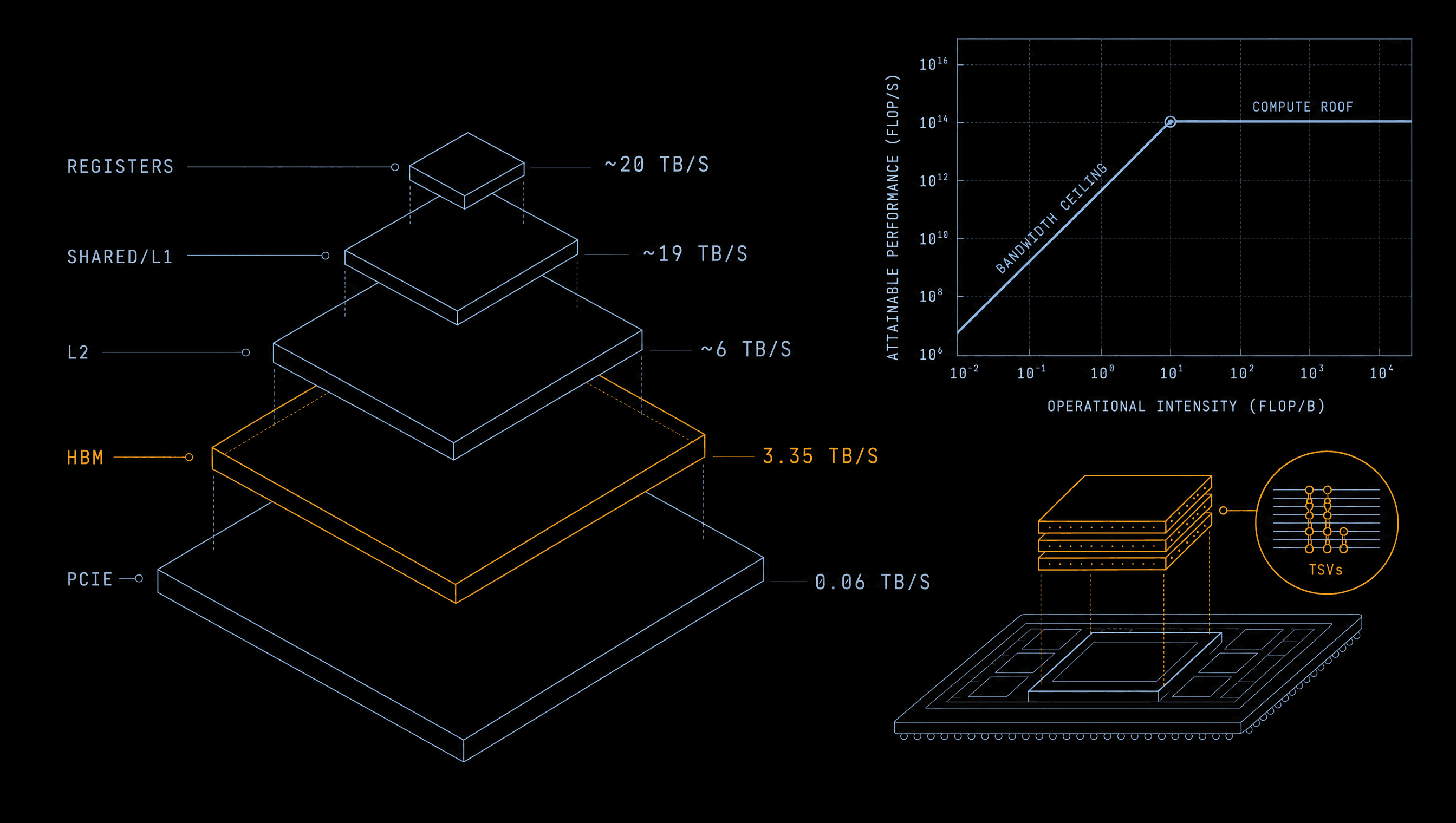
Almost every performance problem in deep learning is a memory problem in disguise: the GPU can do math far faster than it can fetch the numbers to do math on. This chapter builds the model that explains why, and the vocabulary to debug it on a real cluster.
If Chapter 1 was “what the GPU is,” this is “why it's slow.” The most valuable diagnostic instinct an engineer working on GPUs can have is to ask, of any kernel or any workload, a single question: are we bound by compute or by memory? The roofline model makes that question precise, and the answer reorganises every optimization that follows.
The hierarchy, with real bandwidths
Capacity trades against speed, roughly an order of magnitude per tier.
A GPU's memory is a hierarchy of tiers that trade capacity for speed. As you move outward from the arithmetic units, each tier is roughly an order of magnitude larger and an order of magnitude slower. The whole game of GPU optimization is keeping the data you're actively working on in the fast inner tiers and minimising trips to the slow outer ones.
Three of these tiers are worth dwelling on, because you will name them constantly:
Shared memory is the GPU's superpower. It is a slice of the on-chip SRAM that the programmer controls explicitly, a software-managed scratchpad, visible to every thread in a block. Unlike a cache, you decide what goes in it and when. The standard optimization pattern is: cooperatively load a tile of data from slow HBM into fast shared memory once, then have all the threads in the block reuse it many times, amortising the expensive HBM read. We'll see this in the tiled matrix multiply below.
L2 cache is shared across all SMs and is the last line of defence before HBM. On H100 it is a large 50 MB, which can hold meaningful working sets and matters for inference, where the same weights are read repeatedly.
HBM (High-Bandwidth Memory) is the GPU's main memory, the “80 GB” or “141 GB” on the datasheet. It is stacked DRAM connected by an extremely wide bus, which is how it reaches multi-terabyte-per-second bandwidth that ordinary DDR cannot. But “multi-terabyte-per-second” is still glacial next to the arithmetic units, and that gap is the whole story of this chapter.
Coalescing: the first rule of HBM
A warp's 32 loads either fuse into one wide transaction or shatter into many.
HBM is read in transactions, chunks of contiguous bytes (typically 32, 64 or 128 bytes), not individual values. When the 32 threads of a warp issue a load, the hardware coalesces their addresses into as few transactions as possible. If those 32 threads access 32 consecutive 4-byte floats, that is one clean 128-byte transaction, fully coalesced, peak bandwidth. If those same 32 threads access scattered addresses, the hardware must issue many separate transactions, most of whose bytes are thrown away, the effective bandwidth collapses to a fraction of peak.
// COALESCED: thread i reads element i. Consecutive threads -> consecutive
// addresses -> the warp's 32 reads fuse into one 128-byte HBM transaction.
__global__ void copy_coalesced(const float* in, float* out, int n) {
    int i = blockIdx.x * blockDim.x + threadIdx.x;
    if (i < n) out[i] = in[i];                 // stride-1: perfect
}

// STRIDED: thread i reads element i*stride. With stride=32, each thread lands
// in a different 128-byte line -> up to 32 transactions for one warp.
// Effective bandwidth can drop ~10-30x for large strides.
__global__ void copy_strided(const float* in, float* out, int n, int stride) {
    int i = (blockIdx.x * blockDim.x + threadIdx.x) * stride;
    if (i < n) out[i] = in[i];                 // scattered: pathological
}
This is why data layout is a first-class performance concern. Storing a batch of vectors so that the threads of a warp naturally walk contiguous memory (structure-of-arrays rather than array-of-structures) can be the difference between 80% and 8% of peak bandwidth, without changing a single arithmetic operation.
Bank conflicts: shared memory's rule
32 banks, 32 lanes, same-bank access serialises, padding fixes it.
Shared memory has its own performance trap. It is divided into 32 banks, one per warp lane, so that 32 threads can each access a different bank simultaneously at full speed. But if two threads in a warp access different addresses that fall in the same bank, those accesses serialise, a two-way bank conflict halves throughput, an N-way conflict cuts it to 1/N. The classic cause is a stride that is a multiple of 32 (so column-major access of a 32-wide tile hits one bank). The classic fix is padding: declare the tile one element wider than needed so the access pattern skews across banks.
// BAD: a 32x32 tile. Column access tile[threadIdx.y][k] for fixed k hits the
// same bank for every row -> 32-way conflict.
__shared__ float tile_bad[32][32];

// GOOD: pad the inner dimension by 1. Now consecutive rows are offset by 33,
// which is co-prime with 32, so column accesses spread across all 32 banks.
__shared__ float tile_good[32][33]; // <-- the "+1 padding" trickConsecutive threads should hit consecutive addresses, so a warp's 32 loads fuse into one wide transaction. Strided or scattered access shatters into many transactions and wastes bandwidth.
The warp's 32 threads should hit 32 different banks. Same-bank access serialises; padding the tile (e.g. [32][33]) skews the pattern across all banks.
Tiled matrix multiply
The canonical optimization: stage data in fast memory, then reuse it.
Matrix multiply is the heart of deep learning, and the tiled-matmul kernel is the teaching example for why shared memory exists. A naïve matmul reads each element of A and B from HBM many times, for an N×N×N multiply, O(N³) HBM reads. The tiled version loads small tiles of A and B into shared memory once, then every thread in the block reuses those tiles for many multiply-accumulates before fetching the next tile. The HBM traffic drops by a factor equal to the tile width, converting a memory-bound kernel into a compute-bound one. (In production you use cuBLAS or CUTLASS, which do this and far more, but you must understand the idea.)
#define TILE 16
// C = A * B, all NxN, row-major. Each block computes one TILExTILE tile of C.
__global__ void matmul_tiled(const float* A, const float* B, float* C, int N) {
    __shared__ float As[TILE][TILE];
    __shared__ float Bs[TILE][TILE];

    int row = blockIdx.y * TILE + threadIdx.y;
    int col = blockIdx.x * TILE + threadIdx.x;
    float acc = 0.0f;

    // March across the K dimension one tile at a time.
    for (int t = 0; t < N / TILE; ++t) {
        // Cooperative load: each thread brings ONE element of A and B from HBM
        // into shared memory. Coalesced because threadIdx.x is the fast index.
        As[threadIdx.y][threadIdx.x] = A[row * N + (t * TILE + threadIdx.x)];
        Bs[threadIdx.y][threadIdx.x] = B[(t * TILE + threadIdx.y) * N + col];
        __syncthreads();                       // all loads done before compute

        // Now do TILE multiply-accumulates entirely from FAST shared memory.
        // Each HBM value loaded above is reused TILE times here.
        #pragma unroll
        for (int k = 0; k < TILE; ++k)
            acc += As[threadIdx.y][k] * Bs[k][threadIdx.x];
        __syncthreads();                       // before overwriting the tiles
    }
    if (row < N && col < N) C[row * N + col] = acc;
}
The arithmetic is identical to the naïve version; the only change is where the data lives during reuse. That single idea, stage data in fast memory and reuse it, generalises all the way up to FlashAttention, and to how you think about feeding GPUs from storage in Chapter 7.
Arithmetic intensity & the roofline
Making compute-bound vs memory-bound quantitative.
Now we make “compute-bound vs memory-bound” quantitative. Define the arithmetic intensity (AI) of a computation as the number of floating-point operations it performs per byte it moves from memory:
\text{arithmetic intensity } I \;=\; \frac{\text{FLOPs performed}}{\text{bytes moved}} \qquad \left[\tfrac{\text{FLOP}}{\text{byte}}\right]Every GPU has a peak compute rate (FLOP/s) and a peak memory bandwidth (bytes/s). Their ratio defines a threshold intensity called the ridge point. Below it, you are memory-bound; above it, compute-bound. Plotting achievable performance against intensity gives the roofline: a diagonal “memory roof” (bandwidth × AI) that rises until it hits the flat “compute roof” (peak FLOP/s).
The roofline is the most useful single diagram in this book because it dictates strategy. If a kernel is memory-bound (left of the ridge), buying more FLOPs does nothing, you must move fewer bytes (fusion, lower precision, better reuse) or move them faster (more bandwidth, i.e. H200). If it is compute-bound (right of the ridge), more or faster math units (Blackwell, FP8/FP4) is exactly the lever. When a fleet of GPUs sits at low utilization, the very first question is which side of the ridge the workload is on, and the sizing arithmetic later in this chapter shows why so much of inference lives stubbornly on the left.
“Our inference is slow, should we buy faster GPUs?” The roofline answer: token generation is memory-bandwidth-bound, at batch size one you read the entire model from HBM for every single token, doing almost no math per byte. A higher-FLOPS GPU barely helps; what helps is higher bandwidth (H200 over H100), bigger batches to amortise the weight reads across more sequences, quantization to move fewer bytes, or a serving stack like vLLM that batches continuously. Measure tokens/sec and batch size before talking hardware. That reframing, from a hardware purchase to a bottleneck diagnosis, is where the real leverage is.
FlashAttention: fusion as a bandwidth play
Raise arithmetic intensity by refusing to touch HBM.
FlashAttention is the most cited example of “raise arithmetic intensity by not touching HBM,” and it deserves to be understood in systems terms. Standard attention computes softmax(QKᵀ)V by materialising the full N×N score matrix in HBM, where N is the sequence length. For long sequences that matrix is enormous, and writing it out and reading it back dominates the runtime, the operation is memory-bound, with traffic scaling as O(N²).
FlashAttention restructures the computation to tile Q, K and V into blocks that fit in shared memory and computes the softmax incrementally (an online-softmax trick that keeps running max/sum statistics) so the full score matrix never has to exist in HBM at all. The result is roughly an order of magnitude fewer HBM accesses, turning a memory-bound kernel into a near-compute-bound one, the same tiling idea as the tiled matmul, applied to attention. The lesson for the systems builder: a huge fraction of real-world speedups come not from faster silicon but from not moving data you don't have to move.
- Tile Q, K, V into blocks sized to fit in on-chip SRAM (shared memory).
- Compute softmax online, block by block, carrying only a running max and running sum.
- The N×N score matrix never materialises in HBM, O(N²) traffic disappears.
- Roughly 10× fewer HBM accesses; the kernel moves rightward on the roofline toward compute-bound.
The online-softmax trick is not hand-waving, it is an exact identity with a short proof, and it is the one piece of real mathematics inside the most important kernel in modern ML. We prove it in full in the math section below.
Sizing model memory
The back-of-envelope calculation behind every capacity conversation.
One of the most common sizing questions in any GPU capacity conversation is “how much GPU memory does it take to train an N-parameter model?” There is a clean back-of-envelope answer, and it is worth being able to walk through it from first principles. Training memory has four components:
| Component | Bytes / param | Why |
|---|---|---|
| Weights (BF16) | 2 | The model itself, in 16-bit |
| Gradients (BF16) | 2 | One per weight, computed in the backward pass |
| Optimizer, FP32 master weights | 4 | Adam keeps a full-precision copy |
| Optimizer, Adam momentum (m) | 4 | First-moment estimate |
| Optimizer, Adam variance (v) | 4 | Second-moment estimate |
| Total (excl. activations) | ≈ 16 | The famous “16 bytes per parameter” |
So a 7B model needs ≈112 GB of state, already more than one 80 GB H100, before a single activation. A 70B model needs ≈1.1–1.2 TB; a 405B model ≈6.5 TB. This is the arithmetic that forces the sharding and parallelism of Chapter 6, it is not an optimization, it is the reason distributed training exists. On top of this base sits activation memory, which scales with batch size × sequence length × hidden size × number of layers and, for large batches and long context, can rival or exceed the weight memory, which is why activation checkpointing (recomputing activations in the backward pass instead of storing them) is a standard lever.
def training_memory_gb(num_params_billions, bytes_per_param=16):
    """Base state for mixed-precision Adam training, excluding activations."""
    return num_params_billions * 1e9 * bytes_per_param / 1e9   # -> GB

for n in [7, 13, 70, 405]:
    gb = training_memory_gb(n)
    h100s = -(-gb // 80)        # ceil divide by 80GB
    print(f"{n:>4}B model: ~{gb:6.0f} GB state  ->  >= {h100s:.0f}x H100 just to hold it")

#    7B model: ~   112 GB state  ->  >= 2x H100 just to hold it
#   13B model: ~   208 GB state  ->  >= 3x H100 just to hold it
#   70B model: ~  1120 GB state  ->  >= 14x H100 just to hold it
#  405B model: ~  6480 GB state  ->  >= 81x H100 just to hold it
Inference memory is much smaller, roughly 2 bytes/param for BF16 weights (or 1 for INT8/FP8, a little over 0.5 for 4-bit NVFP4) plus the KV cache, which grows with batch size × sequence length and often becomes the binding constraint for long-context serving. We size the KV cache precisely in Chapter 9.
The four numbers to keep in your head
State to train with mixed-precision Adam, derive it from 2+2+4+4+4, don't recite it.
H100 roofline ridge point: peak BF16 compute divided by peak HBM bandwidth.
Arithmetic intensity of batch-1 decode, deep in memory-bound territory, ~40× left of the ridge.
State to train a 70B model, the number that forces sharding and distributed training.
The math: roofline algebra
The roofline as an equation you can evaluate, and the proof inside FlashAttention.
So far the roofline has been a picture. Here it becomes an equation you can differentiate, evaluate, and use to predict the exact dimension at which a matrix multiply flips from memory-bound to compute-bound. Let P be attainable performance (FLOP/s), \beta the peak memory bandwidth (B/s), \pi the peak compute (FLOP/s), and I the arithmetic intensity (FLOP/byte) of the kernel. A kernel can run no faster than its data arrives (\beta I) and no faster than the math units allow (\pi). Hence:
P(I) \;=\; \min\bigl(\pi,\; \beta\, I\bigr)
\beta I that rises with intensity, clamped by a flat “compute roof” \pi. The corner where they meet is the ridge point.Set the two terms equal to find the ridge point I^\star, the arithmetic intensity above which you become compute-bound:
- At the ridge the two roofs are equal:
\beta I^\star = \pi. Below it,\beta I < \pi(memory-bound); above it,\pi < \beta I(compute-bound). - Solve:
I^\star = \pi / \beta. The ridge is simply peak FLOPs divided by peak bandwidth, a property of the hardware, not the kernel. - H100:
\pi \approx 989\times10^{12}FLOP/s (BF16 dense),\beta = 3.35\times10^{12}B/s\Rightarrow I^\star \approx 295FLOP/byte, the ≈295 in FIG 2.2. - A100:
\pi \approx 312\times10^{12},\beta = 2.0\times10^{12} \Rightarrow I^\star \approx 156. H200: same\pias H100 but\beta = 4.8\times10^{12} \Rightarrow I^\star \approx 206, H200's higher bandwidth lowers its ridge, so more workloads become compute-bound. It helps memory-bound work, exactly as Chapter 1 argued.
I^\star \;=\; \frac{\pi}{\beta} \qquad\Rightarrow\qquad I^\star_{\text{H100}} \approx \frac{989\times10^{12}}{3.35\times10^{12}} \approx 295\ \tfrac{\text{FLOP}}{\text{byte}}\pi \approx 2.25\times10^{15}, \beta \approx 8\times10^{12}) gives I^\star \approx 281, Blackwell scales compute and bandwidth together, keeping the machine's balance similar; the gains come from raw magnitude, and from FP8/FP4 shrinking the bytes side. (Figures are a 2026 snapshot, the division is what endures.)| GPU | π (peak BF16 dense) | β (HBM bandwidth) | Ridge I★ = π/β |
|---|---|---|---|
| A100 | 312 × 10¹² FLOP/s | 2.0 × 10¹² B/s | ≈ 156 FLOP/byte |
| H100 | 989 × 10¹² FLOP/s | 3.35 × 10¹² B/s | ≈ 295 FLOP/byte |
| H200 | 989 × 10¹² FLOP/s | 4.8 × 10¹² B/s | ≈ 206 FLOP/byte |
| B200 | ~2.25 × 10¹⁵ FLOP/s | ~8 × 10¹² B/s | ≈ 281 FLOP/byte |
The arithmetic intensity of a GEMM. The most useful intensity to be able to derive on demand is that of a matrix multiply, because it tells you exactly when a layer is compute- or memory-bound. Consider C = AB with A \in \mathbb{R}^{M \times K}, B \in \mathbb{R}^{K \times N}, elements of b bytes. Each of the MN output elements is a length-K dot product, K multiplies plus K adds, i.e. 2K FLOPs, so total FLOPs = 2MNK (the factor of 2 is the universal multiply-and-add convention). Bytes moved, reading A and B and writing C each exactly once, are (MK + KN + MN)\,b, the best case, approached by the tiled matmul we built above.
I_{\text{GEMM}} \;=\; \frac{2MNK}{(MK + KN + MN)\,b}M = N = K = n it collapses to I = \frac{2n^3}{3n^2 b} = \frac{2n}{3b}, intensity grows linearly with the matrix dimension. Big matmuls are compute-bound; small ones are memory-bound. Size decides the side of the ridge.Worked example, the n ≈ 885 crossover. At what size does a BF16 matmul become compute-bound on H100? Set the square-GEMM intensity equal to the ridge and solve for n, with b = 2 bytes (BF16):
\frac{2n}{3b} = I^\star \;\Rightarrow\; n = \frac{3\, b\, I^\star}{2} = \frac{3 \times 2 \times 295}{2} \approx 885So a square BF16 matmul becomes compute-bound around n \gtrsim 885. Check the extremes: n = 4096 \Rightarrow I = 2(4096)/6 \approx 1365 \gg 295 (firmly compute-bound); n = 128 \Rightarrow I \approx 43 \ll 295 (memory-bound). This is why tiny matmuls (small batches, narrow layers, the per-token GEMM in decode) are memory-bound while training's large GEMMs are compute-bound, a single formula predicts both.
Worked example, a real FFN layer. A transformer FFN multiplies activations X \in \mathbb{R}^{M \times K} (M = batch·seq = 8192, K = 4096) by W \in \mathbb{R}^{K \times N} (N = 16384) in BF16. Numerator: 2 \cdot 8192 \cdot 16384 \cdot 4096 \approx 1.10\times10^{12} FLOPs. Denominator bytes: MK = 3.36\times10^{7}, KN = 6.71\times10^{7}, MN = 1.34\times10^{8}; the sum is \approx 2.35\times10^{8} elements, times b = 2 \Rightarrow 4.69\times10^{8} bytes. So I \approx 1.10\times10^{12} / 4.69\times10^{8} \approx 2{,}340 FLOP/byte \gg 295, firmly compute-bound, as expected for a large training GEMM.
I = 2MNK / ((MK+KN+MN)·b) toward the compute roof. This is the quantitative reason batching rescues memory-bound inference: it literally slides the operating point rightward past the ridge.The N = 1 decode result. Now take the tall-skinny extreme: N = 1, a matrix–vector product, exactly what batch-1 decode does at every layer. For M, K \gg 1 the MK term dominates the denominator:
N = 1:\qquad I = \frac{2MK}{(MK + K + M)\,b} \;\xrightarrow{\;M,K \gg 1\;}\; \frac{2}{b} \;\overset{\text{BF16}}{=}\; 1\ \tfrac{\text{FLOP}}{\text{byte}}K, essentially the worst possible, far left of the ridge. This is the formal statement that matrix–vector products are memory-bound: batch-1 decode reads the whole weight matrix to produce one output vector, doing about one FLOP per byte. Batching (raising N) is the only escape, it amortises the weight read across many vectors.The arithmetic intensity of attention. Self-attention computes S = QK^\top, P = \text{softmax}(S), O = PV for sequence length N and head dimension d. Compute: QK^\top is 2N^2 d FLOPs; PV is another 2N^2 d, total \approx 4N^2 d. Naïve HBM traffic: write then read the N \times N scores S and probabilities P,\Theta(N^2)\,b bytes dominate for large N. Hence:
I_{\text{attn}} \;\approx\; \frac{4N^2 d}{\Theta(N^2)\, b} \;=\; \Theta\!\left(\frac{d}{b}\right) \quad\text{— independent of } N.Adding sequence length adds equal compute and memory, so intensity plateaus at a low value set by the head dimension. With d of order 10^2 and b = 2, I_{\text{attn}} sits well below the ridge, attention is memory-bound, and gets more dominated by the N^2 HBM traffic as context grows. FlashAttention tiles Q, K, V into SRAM and never writes S to HBM: the traffic drops from \Theta(N^2) to \Theta(N^2 d / M_{\text{sram}}), reduced by the on-chip reuse factor, which multiplies the effective intensity by that same factor and pushes the operating point toward the compute roof. The mechanism is identical to the tiled-GEMM reuse argument; only the kernel differs.
The online-softmax proof, the heart of FlashAttention. Tiling attention requires computing softmax incrementally, block by block, without ever seeing all scores at once, and doing so without overflow. The proof that this is both numerically safe and exactly correct is worth knowing in full. Step 1 is the safe-softmax identity: direct softmax overflows because e^{x_i} explodes, but subtracting the maximum m = \max_j x_j is provably identical:
\frac{e^{x_i}}{\sum_j e^{x_j}} \;=\; \frac{e^{x_i}}{\sum_j e^{x_j}} \cdot \frac{e^{-m}}{e^{-m}} \;=\; \frac{e^{x_i - m}}{\sum_j e^{x_j - m}}, \qquad m = \max_j x_jx_i - m \le 0, so e^{x_i - m} \in (0, 1]: no overflow. Numerator and denominator are scaled by the same constant, so the value is unchanged.Step 2 merges two blocks correctly. Process the keys in blocks. Suppose block A has already been summarised by a running max m_A, a running denominator \ell_A = \sum_{j \in A} e^{x_j - m_A}, and an accumulated output O_A = \sum_{j \in A} e^{x_j - m_A} v_j. A new block B arrives with its own m_B, \ell_B, O_B. We must combine them as if both had been normalised to the common max m = \max(m_A, m_B). The key observation is that a partial sum computed relative to m_A is converted to be relative to m by multiplying by e^{m_A - m}, the same scale-by-a-constant identity as Step 1, applied to a partial sum:
\sum_{j \in A} e^{x_j - m_A}\, e^{m_A - m} \;=\; \sum_{j \in A} e^{x_j - m}m = \max(m_A, m_B), \qquad \ell = \ell_A\, e^{m_A - m} + \ell_B\, e^{m_B - m}, \qquad O = O_A\, e^{m_A - m} + O_B\, e^{m_B - m}The final attention output is \text{Attn} = O / \ell. Telescoping the updates over all blocks yields
\text{Attn} \;=\; \frac{O}{\ell} \;=\; \frac{\sum_j e^{x_j - m}\, v_j}{\sum_j e^{x_j - m}}, bit-for-bit the safe-softmax result of Step 1. The order of blocks doesn't matter; the running rescale guarantees the streamed result equals the all-at-once result, with no overflow and O(N) memory instead of O(N^2). And the scheme is robust in the extreme case: if block B has a much larger max (m_B \gg m_A), the new max is m = m_B, block A's rescale factor e^{m_A - m_B} is \le 1 and tiny, correctly down-weighting A's negligible scores, block B's factor is exactly 1, and no exponent is ever positive, so nothing overflows. The max-tracking is precisely what keeps every exponent \le 0.
The bandwidth–latency product, revisited. Chapter 1's math used Little's Law L = \lambda W, with memory bandwidth as the arrival rate, to find the parallelism needed to saturate memory. It reappears here as the reason the memory roof has the slope it does: a kernel only reaches \beta I if it sustains enough outstanding requests (\approx \beta W bytes in flight) to hide latency. A kernel that is “on the roofline diagonal” in theory but has too little memory-level parallelism in practice runs below the diagonal, the roofline is an upper bound, and Little's Law tells you whether you can reach it.
\text{ceiling: } P \le \min(\pi,\ \beta I) \qquad\quad \text{reachability: } \text{requests in flight} \;\ge\; \frac{\beta W}{\text{bytes per request}}Self-test
Work these before moving on, each one exercises the roofline instinct.
Q. A cluster's training GPUs show 95% “GPU utilization” in nvidia-smi but the model trains slowly. What is the first hypothesis?
A. That the kernels are memory-bound: the SMs are busy issuing memory instructions and waiting, so the utilization counter reads high, but the arithmetic units (and therefore real throughput) are starved. Put the workload on the roofline, compute the arithmetic intensity, compare to the ridge, and check the true SM/Tensor-Core efficiency and achieved memory bandwidth with profiling, not the coarse utilization metric. Crucially, nvidia-smi “utilization” only means “a kernel was running,” not “the GPU was doing useful math”, a distinction made precise in Chapter 10.
Q. Why does FlashAttention make attention faster without changing the math?
A. Because it stops moving data it doesn't need to move. Standard attention writes the N×N score matrix to HBM and reads it back, O(N²) bandwidth that dominates for long sequences and makes the kernel memory-bound. FlashAttention tiles Q/K/V into shared memory and computes softmax online, so the score matrix never materialises in HBM, roughly 10× fewer HBM accesses, moving the kernel rightward on the roofline toward compute-bound. Same FLOPs, far less memory traffic.
Q. Estimate the memory to train a 13B model, and the number of H100s that implies.
A. About 16 bytes per parameter for mixed-precision Adam, 2 for BF16 weights, 2 for gradients, and 12 for the optimizer's FP32 master copy plus the two Adam moments. 13B × 16 ≈ 208 GB just for state, so at least three 80 GB H100s before any activations, and activation memory at a real batch size and sequence length pushes it higher, which is why the model would be sharded with FSDP or tensor parallelism. The sequence length and batch size are needed to finish the activation estimate. Deriving 16 from its parts, rather than reciting it, is what shows the model is actually understood.
A kernel reads a 32×32 float tile in shared memory column-wise and throughput collapses. What happened, and what is the classic fix?
And remember the distinction underneath that question: coalescing is about global/HBM access, you want the 32 threads of a warp to hit 32 consecutive addresses so they fuse into one wide transaction. Bank conflicts are about shared memory, it has 32 banks, and you want the warp's 32 threads to hit 32 different banks; same-bank access serialises, fixed by padding the tile (e.g. [32][33]). Different memories, different rules.
You now have the two foundations, the execution model and the memory model, that every higher layer assumes. Chapter 3 puts a programming interface on them: how CUDA exposes the GPU to software, and the library and driver stack you will reason about in any real deployment.
- 1Ask first, of any kernel: compute-bound or memory-bound? The roofline P(I) = min(π, βI) makes it precise; the ridge I★ = π/β sits at ≈295 FLOP/byte on H100, ≈156 on A100, ≈206 on H200.
- 2The hierarchy trades capacity for speed, each step outward is ~10× slower and ~100× larger. Keep hot data in registers and shared memory, minimise HBM trips, and never cross PCIe in the inner loop.
- 3Two rules, two memories: coalescing (HBM, consecutive threads hit consecutive addresses) and bank conflicts (shared memory, 32 threads hit 32 different banks; pad [32][33]).
- 4Tiling, staging data in shared memory and reusing it, is the single idea behind both the classic matmul optimization and FlashAttention, whose online softmax is exactly correct by the rescale-and-accumulate proof.
- 5GEMM intensity is 2MNK/((MK+KN+MN)b): square BF16 matmuls cross the H100 ridge at n ≈ 885, while N=1 decode collapses to ~1 FLOP/byte, the formal reason batch-1 inference is bandwidth-bound.
- 6Training with Adam costs ≈16 bytes/param, 112 GB for 7B, ~1.1 TB for 70B, the arithmetic that forces the distributed training of Chapter 6.
Chapters 3 to 12: The Machine, the Cluster, the Platform
Unlock the CUDA software stack, interconnect and collectives, distributed training at scale, storage, orchestration, inference, operations, GPU-cloud economics, and the question bank — each chapter with its math companion woven in.
Join The Agent Foundry to unlock chapters 3 to 12 (the CUDA software stack, interconnect, distributed training, storage, orchestration, inference, operations, GPU-cloud economics), Volume II with the optimization ladder, and every future book on release.
Enter your email to continue. We'll send a one-click sign-in link and bring you back here.
Volume II — The Kernel: one matmul at four altitudes
Unlock the whole of Volume II — one naive CUDA matrix multiply read as source code, user space, kernel space, and silicon, then the optimization ladder (coalescing → shared-memory tiling → register tiling → Tensor Cores), FlashAttention, the end-to-end system diagram, and the appendices.
Join The Agent Foundry to unlock chapters 3 to 12 (the CUDA software stack, interconnect, distributed training, storage, orchestration, inference, operations, GPU-cloud economics), Volume II with the optimization ladder, and every future book on release.
Enter your email to continue. We'll send a one-click sign-in link and bring you back here.