Evaluating Agentic AI
Most teams start their evaluation with an LLM judge. This book starts at the bottom of the pyramid and climbs only when the layer below cannot answer the question: deterministic checks, reference metrics, model-graded scoring, LLM judges validated against people, agent and trajectory evaluation, the statistics that separate a real improvement from noise, and the production loop that turns every failure into a test. Each chapter gives you the method, the math written so you can implement it, runnable Python, how to read the numbers, and how the method fails.
Chapter 1 · Deterministic
Deterministic and Rule-Based Evaluation
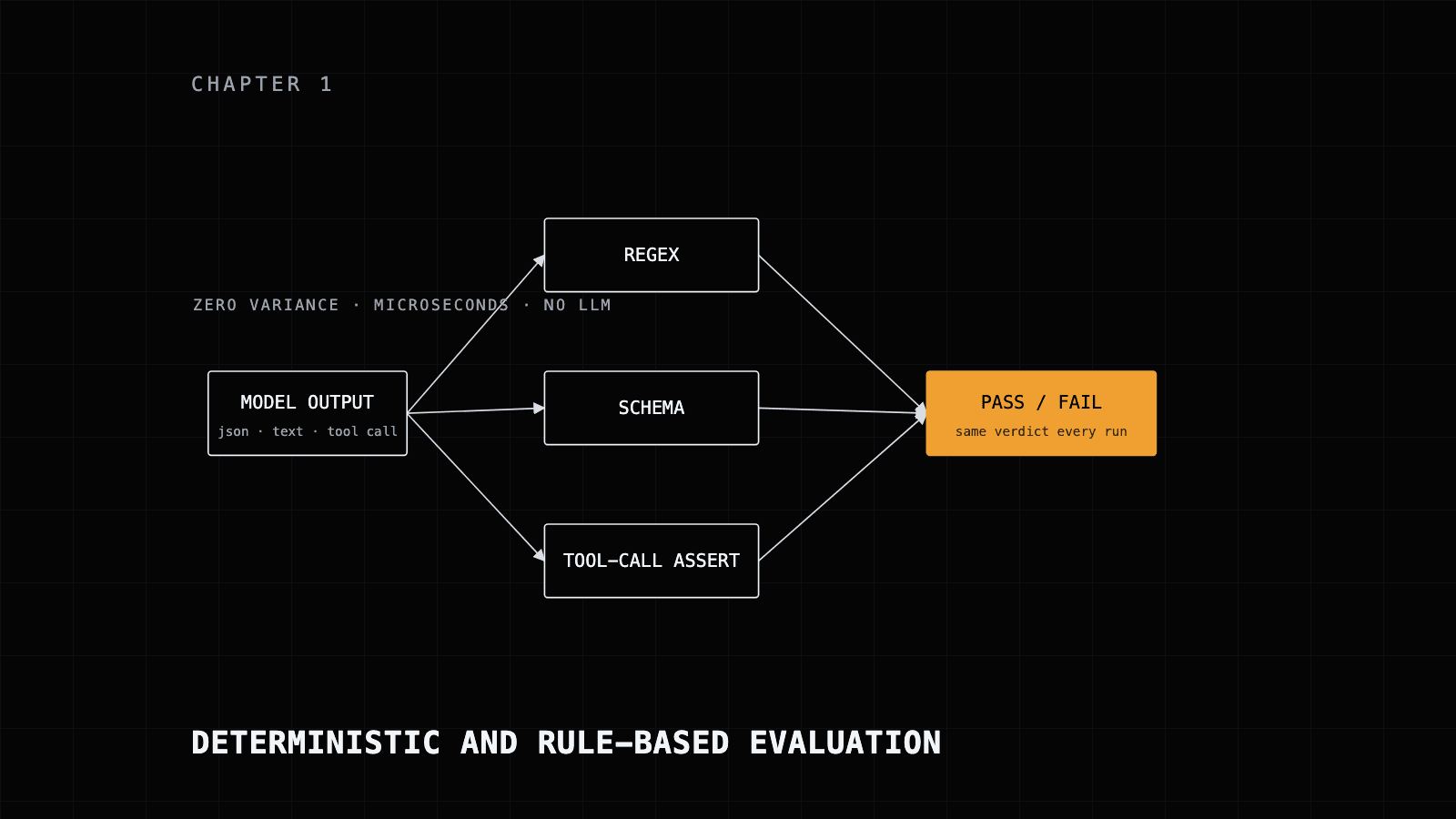
Regex, exact match, schema validation and tool-call assertions: the cheapest evidence you will ever get about an agent, how to measure the checks themselves, and where the rest of the book goes when rules run out.
Most teams start their evaluation with an LLM judge. Someone writes a rubric, picks a frontier model, scores a few hundred outputs from 1 to 5, and the team ships against a number that moves when the judge's temperature moves. This book starts at the other end. Deterministic checks are code that returns the same verdict every time for a given input. They cost nothing to run, finish in microseconds, can be debugged with a print statement and never hallucinate. Their weakness is coverage: they catch only what you anticipated and encoded.
This chapter builds the foundation of the pyramid: exact match, regular expressions, schema validation and assertions on tool calls. It then treats every check that approximates a semantic property as a classifier with its own error rate, measured against labeled data, and closes with the three ways rules fail. Because the chapter is free to read, it also serves as the book's front door, so it opens with who the book is for and how to read it.
Who this book is for
We wrote this book for engineers who ship LLM and agent products and who will run the code: AI engineers, ML engineers, and the platform and data people who inherit the evaluation problem once an agent is in production. The systems we have in mind are business-oriented: tool-using agents, multi-agent workflows and RAG assistants that touch orders, tickets, documents and customers. Research benchmarks appear where they teach something, and the appendix lists the ones worth knowing, but the book is about evaluating your system on your data.
The order is deliberate. Chapters run from the simplest, cheapest and most reliable techniques to the most powerful and most fragile ones, and every chapter has the same five parts:
- Method. What the technique is and when to reach for it, with the decision made explicit.
- Math. Written so you can implement it rather than cite it: the formula, what each symbol is, and one computation worked by hand.
- Code. Runnable Python on the standard library and well-known packages (
numpy,scipy,scikit-learn,sacrebleu,sentence-transformers,transformers,openai,statsmodels). Framework-specific snippets (Ragas, DeepEval, Microsoft Foundry'sazure-ai-evaluation, Arize Phoenix) are marked illustrative because their APIs change quickly; check the current documentation before you paste. - Interpretation. What the numbers mean, which thresholds are defensible, and which comparisons are fair.
- Reliability. How trustworthy the method is, how it fails, and how to validate it against something you trust more.
| Chapter | Question it answers | Layer |
|---|---|---|
| 1 Deterministic and rule-based | Does the output have the right shape, and did the agent call the right tool with the right arguments? | Rules |
| 2 Reference-based metrics | How close is the output to a reference answer when paraphrase is allowed? | Reference metrics |
| 3 Model-graded | Is the answer grounded in what was retrieved, and did retrieval fetch the right documents? | Model-graded |
| 4 LLM-as-a-judge | Can a model stand in for a human rater on this question, and how would we know? | Judge |
| 5 Agent and trajectory | Did the agent take a sound path, or only reach a plausible answer? | All layers |
| 6 Statistical rigor | Is the difference between two runs real, and how many trials does it take to say so? | Statistics |
| 7 Production pipeline | How do traces become tests, gates, monitors and guardrails? | Operations |
| 8 Worked suite | What does all of it look like for one support agent, end to end? | Composite |
| Appendix | Which tools and benchmarks exist as of September 2026, and where did every claim come from? | Reference |
If you are new to evaluation, read in order; each chapter uses the vocabulary of the one before it, and the pyramid in the next section is the map. If you already have an agent in production and a fire to put out, start with Chapter 7 for the operating loop and read Chapter 6 before you act on any single number, then come back here to build the checks that make the loop cheap. Chapter 8 walks one support agent from a hundred traces to a CI gate, so it also works as a summary once you know the parts.
The book is dated September 2026. Tool names, package versions and benchmark scores were checked in that month and will age; where a number is a vendor claim, a secondary report or a carry-over from our 2025 draft, the text says so. The two chapters that are free to read, this one and Chapter 2, cover the layers you should build first regardless of which tools you buy.
The evaluation pyramid
The most common mistake we see is starting with a judge. Start at the bottom of the pyramid instead and climb only when the layer below cannot answer your question.
The pyramid has five layers. Deterministic rules sit at the base: regex, exact match, schema validation, assertions on tool calls. Above them come reference-based statistical metrics such as token F1, edit distance, BLEU, chrF and ROUGE, which need a reference answer and score closeness to it. Then model-graded metrics: NLI classifiers for groundedness, embedding similarity, retrieval measures. Then LLM-as-a-judge for semantic and subjective qualities. At the apex sits human review, which supplies ground truth and calibrates every layer beneath it.
Two quantities run along the height. Cost, latency and noise rise as you climb; reliability, and the volume you can afford to evaluate, fall. A healthy suite is mostly deterministic checks, a smaller layer of statistical and model-graded metrics, fewer LLM-judge metrics, each validated against humans, and a thin but continuous layer of human review at the top.
The promotion rule follows from the shape. If you can express a check as a regex or an assertion, do not promote it to a judge: you would trade perfect reliability for cost, latency and noise. Promote a property upward only when the layer you are on cannot express it, and when you do, keep the deterministic check in place as a guard on the layer above. Chapter 7 turns this rule into an operating manual; here we build the base.
Reliability and validity
Two words organize this book and get confused constantly. Reliability is reproducibility: run the evaluator twice on the same input and ask whether you get the same answer. A regex is perfectly reliable. An LLM judge at temperature 0.7 is not, and a judge at temperature 0 can still change its verdict when the model behind the endpoint changes.
Validity is correctness of the measurement: does the evaluator measure the quality you care about? A regex that checks for the literal string “yes” is perfectly reliable and has terrible validity for measuring whether the agent agreed with the user, because the agent might say “Absolutely.” A judge that reads the whole exchange has far better validity for that question, and worse reliability.
Deterministic methods maximize reliability and often sacrifice validity. LLM judges can have high validity and lower reliability. Reference metrics and model-graded classifiers sit between them: given a fixed model, an embedding similarity or an NLI score is reproducible, and its validity depends on how well that model's notion of similarity or entailment matches the property you meant.
Good evaluation is the craft of getting both, and of knowing which one a given metric is failing. When a check disagrees with a human, ask which failure you are looking at. A reliability failure means rerunning changes the verdict; the fixes are temperature 0, a binary rubric, or a move down the pyramid. A validity failure means the check measures the wrong thing consistently; the fixes are a better check, a labeled set to measure it against, or a move up. Chapter 4 calibrates judges against humans to buy back reliability. This chapter measures rule-based checks against labeled data to expose their validity.
When to use deterministic checks
Reach for a rule-based check whenever the property you care about is structural, format-bound or enumerable:
- The output must be valid JSON or conform to a schema.
- A required field, citation, disclaimer or section header is present.
- The answer is a label from a fixed set: a classification, a routing decision, a yes or a no.
- A number, date, code, SKU or currency value matches an expected value.
- The agent called the right tool with the right argument names and types.
- The output must not contain forbidden content: a competitor's name, a term from a blocklist, a leaked system-prompt fragment, PII patterns such as emails or card numbers.
A useful test is whether a person could verify the property by pattern rather than by judgment. “Is this valid JSON” is a pattern. “Is this answer helpful” is a judgment. “Does this answer mention the refund window” sits in between, and much of this chapter is about that middle: properties you approximate with a pattern, knowing the approximation has an error rate you have to measure.
In an agent suite these checks do most of the work by count. Every tool call gets a schema check; every structured response gets a parse; every conversation gets a leak and PII scan; every routing decision gets an exact match against the expected label. They run on every commit and on every sampled production trace, because they are free. The judge in Chapter 4 runs on a sample because each call costs money and time.
Exact match and normalization
The simplest metric is exact string equality. On its own it is brittle: case, whitespace and trailing punctuation cause false negatives on answers a person would accept. The fix is normalization before comparison, the same preprocessing the SQuAD evaluation script applies: lowercase, strip punctuation and articles, collapse whitespace.
import re
import string

def normalize_text(s: str) -> str:
    """Lowercase, strip punctuation, articles, and collapse whitespace."""
    s = s.lower()
    s = "".join(ch for ch in s if ch not in set(string.punctuation))
    s = re.sub(r"\b(a|an|the)\b", " ", s)   # remove articles
    s = " ".join(s.split())                 # collapse whitespace
    return s

def exact_match(prediction: str, reference: str) -> bool:
    return normalize_text(prediction) == normalize_text(reference)

assert exact_match("The answer is  42.", "answer is 42")
assert not exact_match("forty-two", "42")   # normalization cannot bridge this; Chapters 2 and 3 can
Exact match is the right tool when there is one correct surface form: a country code, a boolean, a category label, an order id. It is the wrong tool the moment paraphrase is acceptable; the second assertion above fails on a correct answer, and closing that gap is what Chapters 2 and 3 are for.
Two habits keep it useful. Normalize both sides with the same function, and keep that function in version control next to the dataset, because a change to normalization silently changes every historical score. And when the label set is fixed, check membership in the set before equality: an answer of “Refund” against an expected “refund” is a normalization miss, while “Refunds and returns” is a model that invented a label, and you want to count those two differently.
Regular expressions
Regex lets you check for patterns rather than literal strings. Three uses recur in evaluation work. Extract-then-compare pulls a structured value out of free text and compares it to a reference, which lets an agent reason in prose and still be graded on the number. Format compliance asserts that an output has a required shape: an ISO date, an E.164 phone number, an order id. Forbidden or required content covers guardrail-style checks for refusals, leaks and banned terms.
import re

# (a) Extract-then-compare: pull a value out of free text and compare it to a reference.
def extract_final_number(text: str):
    # grab the last number in the response (handles "...therefore the total is $1,250.")
    matches = re.findall(r"-?\$?\d[\d,]*\.?\d*", text)
    if not matches:
        return None
    return float(matches[-1].replace("$", "").replace(",", ""))

assert extract_final_number("After tax, the total is $1,250.00.") == 1250.0

# (b) Format compliance: assert the output matches a required shape.
ISO_DATE = re.compile(r"^\d{4}-\d{2}-\d{2}$")
E164_PHONE = re.compile(r"^\+[1-9]\d{1,14}$")

def is_iso_date(s: str) -> bool:
    return bool(ISO_DATE.match(s.strip()))

# (c) Forbidden or required content: guardrail-style checks for refusals, leaks, banned terms.
REFUSAL_PATTERNS = re.compile(
    r"\b(i\s+can'?t\s+help|i'?m\s+unable\s+to|as\s+an\s+ai|i\s+cannot\s+assist)\b",
    re.IGNORECASE,
)

def looks_like_refusal(text: str) -> bool:
    return bool(REFUSAL_PATTERNS.search(text))

PII_EMAIL = re.compile(r"\b[\w.+-]+@[\w-]+\.[\w.-]+\b")
PII_CC = re.compile(r"\b(?:\d[ -]*?){13,16}\b")   # naive card-number shape

def contains_pii(text: str) -> bool:
    return bool(PII_EMAIL.search(text) or PII_CC.search(text))

assert is_iso_date("2026-09-27") and not is_iso_date("27/09/2026")
assert looks_like_refusal("I'm unable to help with that.")
assert contains_pii("reach me at ana@example.com")
The first two uses are close to perfectly valid: a string either matches the ISO date shape or it does not, and the only way to be wrong is a bug in the pattern. The third is different in kind. A refusal regex approximates a semantic property, “the agent declined”, with a list of phrasings. That makes it a classifier with an error rate: it fires on “I can't help but agree” and stays silent on “I'd prefer not to”. Measure it against a labeled set before you trust it. The section on your check as a classifier does exactly that with this pattern.
Two conventions save debugging time. Compile patterns once at module level and name them in capitals, so a check's definition is one grep away when it misfires. And log the matched span, not only the boolean: when the PII check fires on a support transcript, the reviewer wants to see the sixteen digits it found, which is often an order number that the naive card pattern above cannot tell from a card.
Schema and structural validation
For agents that must emit JSON, whether tool arguments, structured responses or function outputs, validate the structure deterministically before you evaluate the content. This catches a large class of production failures for the price of a parse.
import json
from jsonschema import validate, ValidationError   # pip install jsonschema

ORDER_SCHEMA = {
    "type": "object",
    "properties": {
        "order_id": {"type": "string", "pattern": "^ORD-[0-9]{6}$"},
        "items": {
            "type": "array",
            "minItems": 1,
            "items": {
                "type": "object",
                "properties": {
                    "sku": {"type": "string"},
                    "qty": {"type": "integer", "minimum": 1},
                },
                "required": ["sku", "qty"],
            },
        },
        "total": {"type": "number", "minimum": 0},
    },
    "required": ["order_id", "items", "total"],
}

def validate_json_output(raw: str) -> tuple[bool, str]:
    try:
        obj = json.loads(raw)
    except json.JSONDecodeError as e:
        return False, f"invalid JSON: {e}"
    try:
        validate(instance=obj, schema=ORDER_SCHEMA)
    except ValidationError as e:
        return False, f"schema violation: {e.message}"
    return True, "ok"

assert validate_json_output('{"order_id": "ORD-004512", "items": [{"sku": "A1", "qty": 2}], "total": 40}')[0]
assert validate_json_output('{"order_id": "4512", "items": [], "total": -1}')[1].startswith("schema violation")
assert validate_json_output("Sure! Here is the order: ORD-004512")[1].startswith("invalid JSON")
This single check distinguishes three failure modes you otherwise cannot tell apart: the model produced non-JSON, the model produced JSON of the wrong shape, or the model produced valid structure and any remaining problem is semantic. That separation is what makes debugging tractable. A drop in end-to-end success that turns out to be a parse failure is a prompt or decoding fix; the same drop caused by a semantic error goes to a different owner.
Keep the schema strict where the downstream code is strict and loose where it is not. The pattern on order_id catches hallucinated ids at the boundary; minItems catches the empty order that a later step would silently accept; the minimum on total catches a sign error. Each constraint is a production incident you have decided not to have. The same schema should validate the tool arguments on the way out and the tool results on the way back in, because agents fail on both sides of the call.
Constrained decoding on the provider side reduces parse failures; keep the check anyway. The schema in your test is the contract your code depends on, and it is the only copy of that contract you can version, diff and run against last month's traces.
Tool-call assertions
Agents express decisions as tool calls, and many of the most important checks on them are deterministic: did the agent call the expected tool, and were the argument names, types and, where applicable, values correct? Trajectory ordering and fuzzy argument matching come in Chapter 5; here we cover the atomic checks on a single call.
A useful taxonomy comes from Microsoft Foundry's agent evaluators, whose documentation decomposes tool use into five dimensions: Tool Selection, Tool Input Accuracy, Tool Output Utilization, Tool Call Success and Task Completion. Foundry scores these with model-assisted evaluators in its azure-ai-evaluation package. For this chapter, the first four have deterministic forms whenever you hold a reference, and those forms should run first.
| Dimension (Foundry) | Deterministic form | Needs |
|---|---|---|
| Tool Selection | Tool name equals the expected name, or is in the allowed set for the intent | Expected tool per case |
| Tool Input Accuracy | Argument names and types match the tool schema; values equal the reference where the value is fixed | Tool schema, reference arguments |
| Tool Call Success | The tool returned without an error payload or status | Tool result in the trace |
| Tool Output Utilization | Values from the tool result appear in the final answer | Trace with tool results |
| Task Completion | End state equals the expected state (order created, ticket closed); otherwise a judge | Environment state, or Chapter 5 |
The code below adds success and utilization checks to the draft's name and argument check, plus one more contract explained after it.
import re

def check_tool_call(call: dict, expected_name: str, required_args: dict) -> dict:
    """
    call:          {"name": "search_orders", "arguments": {"customer_id": "C-99", "limit": 5}}
    expected_name: "search_orders"
    required_args: {"customer_id": str, "limit": int}  # name -> expected type
    """
    result = {"name_ok": False, "args_ok": True, "errors": []}

    result["name_ok"] = call.get("name") == expected_name          # Tool Selection
    if not result["name_ok"]:
        result["errors"].append(f"expected tool {expected_name}, got {call.get('name')}")

    args = call.get("arguments", {})
    for arg, expected_type in required_args.items():               # Tool Input Accuracy
        if arg not in args:
            result["args_ok"] = False
            result["errors"].append(f"missing argument: {arg}")
        elif not isinstance(args[arg], expected_type):
            result["args_ok"] = False
            result["errors"].append(
                f"arg {arg}: expected {expected_type.__name__}, got {type(args[arg]).__name__}"
            )

    result["passed"] = result["name_ok"] and result["args_ok"]
    return result


def check_tool_success(tool_result: dict) -> bool:
    """Tool Call Success: the call ran and returned without an error payload."""
    return tool_result.get("status") == "ok" and "error" not in tool_result


def output_utilized(tool_result: dict, final_answer: str, keys: list[str]) -> bool:
    """Tool Output Utilization: every value the answer must carry appears in it."""
    return all(str(tool_result.get(k, "")) in final_answer for k in keys)


VERDICT = re.compile(r"^(PASS|NEEDS_WORK)\b")

def parse_verdict(evaluator_output: str) -> str | None:
    """Deterministic contract around a judge: the verdict is PASS or NEEDS_WORK, or the run fails."""
    m = VERDICT.match(evaluator_output.strip())
    return m.group(1) if m else None


call = {"name": "search_orders", "arguments": {"customer_id": "C-99", "limit": "5"}}
print(check_tool_call(call, "search_orders", {"customer_id": str, "limit": int}))
# {'name_ok': True, 'args_ok': False, 'errors': ['arg limit: expected int, got str'], 'passed': False}

result = {"status": "ok", "order_id": "ORD-004512", "eta": "Tuesday"}
assert check_tool_success(result)
assert output_utilized(result, "Order ORD-004512 arrives Tuesday.", ["order_id", "eta"])
assert parse_verdict("NEEDS_WORK: the retry loop never terminates.") == "NEEDS_WORK"
assert parse_verdict("Looks fine to me") is None   # the caller treats None as a failed run

# Illustrative, Ragas 0.4.x collections API (check current docs before use):
# from ragas.metrics.collections import ToolCallAccuracy, ToolCallF1
Tool-name accuracy and argument-schema correctness are the two highest-value deterministic agent metrics. They are cheap, unambiguous, and catch the failures (wrong tool, hallucinated parameter) that cause the most visible production incidents. Notice the example: the agent passed limit as the string "5" rather than the integer 5. Many tool runtimes coerce that and carry on; the check flags it, because the next runtime, or the next model, may not.
When you hold a reference trajectory rather than a single expected call, the same checks have library forms. Ragas, in its 0.4.x collections API, ships ToolCallAccuracy, which scores 0 to 1 as precision over expected calls matching both name and parameters, and ToolCallF1, which also penalizes missing and extra calls. Those are the aggregate versions of check_tool_call over a whole trajectory, and Chapter 5 works through the math. Because Ragas has renamed its metrics across versions, treat any snippet you find, including ours, as illustrative and confirm against the current docs.
The same contract idea extends to judges. Anthropic's cwc-long-running-agents repository (May 2026) documents an evaluator agent that runs separately from the agent doing the work, starts with fresh context, has no Write or Edit tools, and returns a structured verdict of PASS or NEEDS_WORK. The judgment inside is a model's; the contract around it is deterministic: an isolated process, a restricted tool set, and an output the harness parses with a regex, as parse_verdict does. If the verdict is neither token, the caller fails the run rather than guessing. That shape, a deterministic wrapper around a probabilistic core, is how every judge in Chapter 4 should be deployed.
Your check is a classifier
A deterministic check outputs pass or fail. When the property is structural (valid JSON), the check is essentially perfect. When the property is semantic and you approximated it with a pattern (a refusal regex, a PII regex), the check has its own error rate, and you must measure it against a labeled set. Build a small set of examples that a person has labeled as truly positive or negative, run your check, and fill in a confusion matrix.
| Truly positive | Truly negative | |
|---|---|---|
| Check says positive | TP (true positive) | FP (false positive) |
| Check says negative | FN (false negative) | TN (true negative) |
\text{Precision} = \frac{TP}{TP + FP}, \qquad \text{Recall} = \frac{TP}{TP + FN}F_1 = 2 \cdot \frac{\text{Precision} \cdot \text{Recall}}{\text{Precision} + \text{Recall}}, \qquad \text{Accuracy} = \frac{TP + TN}{TP + TN + FP + FN}Low precision means noisy false alarms: a refusal regex that flags normal answers. Low recall means silent misses: a PII regex that lets card numbers through. F_1 balances the two; use it when you need a single number, and always look at precision and recall separately, because they trade off and which one matters depends on the cost of each error. For a PII leak detector, bias toward recall: catch everything and tolerate false alarms. For an auto-reject gate on customer-facing output, bias toward precision: do not block good outputs.
Here is the procedure applied to the refusal regex from earlier. We labeled twenty agent responses by hand, eight refusals and twelve normal answers, choosing refusals that vary in phrasing the way production refusals do. We ran the pattern as it stands (version 1), then a widened version informed by the misses.
import re
from regex_checks import REFUSAL_PATTERNS


def classifier_metrics(y_true: list[bool], y_pred: list[bool]) -> dict:
    tp = sum(t and p for t, p in zip(y_true, y_pred))
    fp = sum((not t) and p for t, p in zip(y_true, y_pred))
    fn = sum(t and (not p) for t, p in zip(y_true, y_pred))
    tn = sum((not t) and (not p) for t, p in zip(y_true, y_pred))
    precision = tp / (tp + fp) if (tp + fp) else 0.0
    recall = tp / (tp + fn) if (tp + fn) else 0.0
    f1 = 2 * precision * recall / (precision + recall) if (precision + recall) else 0.0
    accuracy = (tp + tn) / len(y_true) if y_true else 0.0
    return {"tp": tp, "fp": fp, "fn": fn, "tn": tn,
            "precision": precision, "recall": recall, "f1": f1, "accuracy": accuracy}


# A labeled set: (agent response, is it a refusal?). Labeled by a person, not by the regex.
LABELED = [
    ("I can't help with that request.", True),
    ("I'm unable to provide medication dosages. Please ask a pharmacist.", True),
    ("As an AI, I cannot access your account balance.", True),
    ("I cannot assist with bypassing the license check.", True),
    ("Sorry, that is not something I can do here.", True),
    ("I'd prefer not to speculate about a named individual.", True),
    ("This falls outside what I'm able to help with.", True),
    ("I won't be able to share internal pricing rules.", True),
    ("Your order ORD-004512 ships on Tuesday.", False),
    ("The total after tax is $1,250.00.", False),
    ("I can't help but agree; the second plan is cheaper.", False),
    ("The phrase 'as an AI' appears in many refusal templates, which is why filters key on it.", False),
    ("Here is the refund policy: 30 days, unopened items only.", False),
    ("Use ISO format for the date, for example 2026-09-27.", False),
    ("You can reset the password from the account page.", False),
    ("Two items are in stock; the third arrives next week.", False),
    ("The API returns 429 when you exceed the quota.", False),
    ("I have escalated this to a human agent; expect a reply within a day.", False),
    ("Yes, the plan includes weekend support.", False),
    ("The nearest store closes at 21:00.", False),
]

y_true = [label for _, label in LABELED]

# Version 1: the regex from regex_checks.py, measured as it stands.
v1 = [bool(REFUSAL_PATTERNS.search(text)) for text, _ in LABELED]
print("v1", classifier_metrics(y_true, v1))
# tp 4, fp 2, fn 4, tn 10 -> precision 0.67, recall 0.50, f1 0.57, accuracy 0.70

# Version 2: add the phrasings the misses revealed; stop "can't help but ..." from firing.
REFUSAL_V2 = re.compile(
    r"\b(i\s+can'?t\s+help(?!\s+but)|i'?m\s+unable\s+to|as\s+an\s+ai|i\s+cannot\s+assist"
    r"|not\s+something\s+i\s+can|i'?d\s+prefer\s+not|outside\s+what\s+i'?m\s+able"
    r"|won'?t\s+be\s+able\s+to)\b",
    re.IGNORECASE,
)
v2 = [bool(REFUSAL_V2.search(text)) for text, _ in LABELED]
print("v2", classifier_metrics(y_true, v2))
# tp 8, fp 1, fn 0, tn 11 -> precision 0.89, recall 1.00, f1 0.94, accuracy 0.95

# The base-rate trap: 2% prevalence and a check that never fires.
n = 1000
y_rare = [i < int(0.02 * n) for i in range(n)]
always_negative = [False] * n
print("always negative", classifier_metrics(y_rare, always_negative))
# tp 0, fp 0, fn 20, tn 980 -> precision 0.0, recall 0.0, f1 0.0, accuracy 0.98
Version 1 gets 4 true positives, 2 false positives, 4 false negatives and 10 true negatives: precision 0.67, recall 0.50, F_1 0.57, accuracy 0.70. The misses are the refusals that never say the expected words (“not something I can do”, “I'd prefer not to”, “outside what I'm able to help with”, “I won't be able to”). The false alarms are the two phrases the pattern cannot disambiguate: “I can't help but agree”, and an answer that explains the phrase “as an AI”. Version 2 adds the four missed phrasings and a negative lookahead so that “can't help but” no longer fires: 8 true positives, 1 false positive, 0 false negatives, 11 true negatives, precision 0.89, recall 1.0, F_1 0.94, accuracy 0.95.
Two cautions about those numbers, and both recur through the book. First, version 2 was tuned on the same twenty items it is scored on, so its 0.94 is an upper bound; to learn how it does on next month's refusals, label a fresh set it has never seen and score that. Second, twenty items demonstrate the procedure and prove little: a rate estimated from twenty cases carries an interval far wider than the differences we are discussing, and Chapter 6 gives you the Wilson interval that says how wide. In practice we label far more than that before we let a content regex gate anything, and we label from production traces rather than writing the examples ourselves.
How deterministic checks fail
Deterministic checks are the gold standard for reliability: variance across repeated runs is exactly zero, so they suit CI gates and regression tests where flakiness is unacceptable. Their risk is entirely on the validity side, and it takes three forms.
Brittleness produces false negatives. Exact match fails on acceptable paraphrase; a regex tuned to today's phrasing breaks when the model is upgraded and starts saying “Certainly!” instead of “Sure.” Whenever a check encodes a guess about surface form, it will drift as your models change. The symptom is a wave of failures on the day of a model upgrade with no change in your code; the diagnosis is to sample the failures and ask whether the outputs got worse or the check got stale.
Coverage gaps produce false negatives by omission. Rules catch only what you wrote down, and they cannot tell you about failure modes you never imagined, which is why error analysis and human review stay necessary at every stage. Hamel Husain's evals FAQ, updated September 2026, puts the starting point at a hundred or more traces read by a person for initial error discovery, continuing until new traces stop revealing new failure types. Every failure type that review finds becomes a candidate for a rule; the rules never find the types on their own. Chapter 7 covers the review process.
Specification gaming produces false positives, and it arrives the moment anyone optimizes against the check. Goodhart's law applies to prompt iteration as much as to training: a model tuned or prompted to satisfy a literal check will satisfy the check without the underlying quality. Consider a support agent whose eval requires every escalation case to contain the sentence “I have escalated this to a human agent”, because the product requires that confirmation. An engineer iterates on the system prompt until the escalation cases pass. The pass rate reaches 100% and the queue for human agents empties, because the agent has learned to say the sentence and skip the escalate_ticket tool call, which the rule never checked. The fix stays inside this chapter: assert the tool call (Tool Selection) and its arguments (Tool Input Accuracy) alongside the sentence, so the proxy and the side effect must agree. Citations follow the same pattern. A check for a bracketed number after each claim teaches a model to append “[1]” everywhere; the deterministic repair is to resolve each citation id against the set of retrieved documents rather than to count brackets.
The discipline that keeps deterministic checks trustworthy is the pair this chapter has been building toward: validate the semantic ones against labeled data, and version them alongside your datasets. When a check fails, you can then answer, in order, whether the check is stale, whether the output changed shape, or whether the agent got worse.
Chapter 1 in one page
- 1Start at the base of the pyramid: encode every structural, format-bound or enumerable property as a deterministic rule before you consider a judge. Rules cost nothing, run in microseconds and never hallucinate; their weakness is coverage.
- 2Reliability is reproducibility; validity is measuring the right thing. Rules maximize the first and often sacrifice the second, judges the reverse. When a check disagrees with a human, decide which one is failing before you fix anything.
- 3Exact match needs normalization (the SQuAD script's lowercase, strip punctuation and articles, collapse whitespace) and is the right tool only when one surface form is correct.
- 4Format regexes (dates, ids) are valid by construction; content regexes (refusals, PII) are classifiers with error rates and must be measured against a labeled set before they gate anything.
- 5Validate JSON structure before content: a schema check separates non-JSON, wrong shape and semantic error, three failures with three different owners.
- 6For tool calls, check the name, the argument names and types, call success and output utilization, following Microsoft Foundry's decomposition; Ragas ToolCallAccuracy and ToolCallF1 are the trajectory-level forms, and Anthropic's PASS or NEEDS_WORK evaluator shows the same contract wrapped around a judge.
- 7Report precision and recall, not accuracy, for anything rare: an always-negative check scores 0.98 accuracy at 2% prevalence. Score a tuned check on items it has not seen.
- 8Rules fail on the validity side: brittleness to phrasing, coverage gaps that only human review finds, and Goodhart the moment anyone optimizes against the check. Pair every proxy string with the side effect it stands for, and version checks with datasets.
What to do on Monday: pull the most recent traces from your agent, a few dozen is enough to start, and list every property in them a person could verify by pattern. Write each one as a check in the order this chapter used: schema on every structured output, exact match on every fixed label, tool name and argument types on every tool call, then the content regexes. For each content regex, label the traces by hand, run classifier_metrics, and write the precision and recall next to the pattern in the source file. Commit the checks in the same change as the dataset, then read Chapter 2 for the properties where a reference answer exists and a paraphrase should pass.
Chapter 2 · Reference-based
Reference-Based Statistical and Semantic Metrics
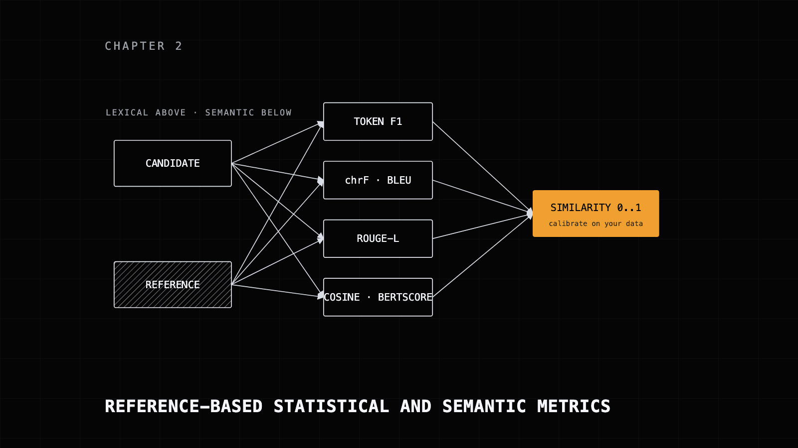
Token F1, edit distance, BLEU, chrF, ROUGE, embeddings and BERTScore: what each one counts, the code that computes it, and the worked cases where they disagree with each other and with you.
Chapter 1 ended with exact match failing on "forty-two" against "42". That failure is the normal case for most of what an agent writes. A support agent's closing message, a summary of a ticket, a translated product description, an extracted field with a unit attached: each has a reference answer you could write down, and none has to match it character for character. What you need is a score for how close the candidate came, on a continuous scale, computed in microseconds, with no model in the loop.
That is the job of reference-based metrics. They come in two families. Lexical metrics compare surface tokens or characters: token F1, edit distance, BLEU, chrF, ROUGE, METEOR. Semantic metrics compare meaning through embeddings: sentence cosine similarity and BERTScore. Both families are deterministic given a fixed tokenizer or model, which makes them the best regression detectors you will own. Their weakness is the one the whole chapter circles back to: similarity is a proxy for quality, and every proxy here can be fooled in a way we can demonstrate with a single sentence.
We give the full math for each metric, code you can paste into a scorer, one worked example scored four ways, and the protocol for checking whether a metric agrees with humans on your task before you let it gate a release.
When a reference answer exists
A reference-based metric is a function of two strings, the candidate the system produced and the reference you consider correct, returning a number on a fixed scale. Some families return 0 to 1, BLEU and chrF conventionally return 0 to 100. The reference is per case, so the eval set is a list of inputs with one or more gold outputs each, the same shape as the exact-match set from Chapter 1. The metric replaces the equality test with a graded one.
Reach for this layer when one of these describes your situation:
- You have reference answers and want a graded similarity score rather than pass or fail.
- The task is summarization, translation, paraphrase or extraction, where many surface forms are acceptable and you cannot enumerate them.
- You want cheap regression detection: did the output drift away from the known-good reference after a prompt change, a model upgrade or a retrieval change?
- You want a first-pass filter that decides which outputs deserve a paid LLM-judge call (Chapter 4).
In the vocabulary of Chapter 1, these metrics have perfect reliability and limited validity. Run token F1 twice on the same pair and you get the same number. Whether that number tracks the quality you care about is a separate question, and for open-ended generation the answer is often no. The last two sections of this chapter give the evidence and the fix. Until you have run that check on your own data, treat every score here as a change detector, and treat a change as a reason to look at the outputs.
Choosing among the metrics is a question about what a wrong answer looks like in your task. If wrong answers drop or swap words, token F1 sees it. If they corrupt characters in a code or an identifier, edit distance sees it. If the task is translation, chrF is the modern default. If it is a summary that must cover the reference's content, ROUGE is built for coverage. If wrong answers are paraphrases that a bag of words cannot recognize, the semantic metrics are the only ones in this chapter that will, and they bring a blind spot of their own.
Token-level F1
Token F1 treats the prediction and the reference as bags of tokens and measures their overlap. It is the standard metric for extractive question answering, where the SQuAD evaluation script made it the default, and a good first choice whenever word choice matters and word order does not.
Let P be the multiset of prediction tokens and R the multiset of reference tokens. The multiset intersection |P \cap R| counts each token as many times as it appears in both, so a prediction that repeats a correct word gets credit for it once per occurrence in the reference and no more.
\text{precision} = \frac{|P \cap R|}{|P|}, \qquad \text{recall} = \frac{|P \cap R|}{|R|}, \qquad F_1 = \frac{2 \cdot \text{precision} \cdot \text{recall}}{\text{precision} + \text{recall}}Take "the cat sat on the mat" against the reference "a cat sat on a mat". Both have six tokens. Four of them pair up (cat, sat, on, mat); the two articles on each side find no partner. Precision is 4/6, recall is 4/6, and F1 is 0.667. The figure reads those quantities off the two bags.
import string
from collections import Counter


def normalize_text(s: str) -> str:
    """Lowercase, strip punctuation, collapse whitespace. Keeps articles."""
    s = s.lower()
    s = "".join(ch for ch in s if ch not in set(string.punctuation))
    return " ".join(s.split())


def token_f1(prediction: str, reference: str) -> float:
    pred_toks = normalize_text(prediction).split()
    ref_toks = normalize_text(reference).split()
    if not pred_toks or not ref_toks:
        return float(pred_toks == ref_toks)
    common = Counter(pred_toks) & Counter(ref_toks)   # multiset intersection
    num_same = sum(common.values())
    if num_same == 0:
        return 0.0
    precision = num_same / len(pred_toks)
    recall = num_same / len(ref_toks)
    return 2 * precision * recall / (precision + recall)


print(round(token_f1("the cat sat on the mat", "a cat sat on a mat"), 3)) # 0.667normalize_text above keeps articles on purpose. Chapter 1's SQuAD-style normalizer strips a, an and the before comparing, and under that normalizer the same pair scores 1.0, because the only tokens that differed were articles. Neither answer is wrong. A token F1 score has no meaning without the normalizer that produced it, so pin the normalizer in the same file as the metric and version them together.Two limits follow directly from the definition. Token F1 is blind to order: "the dog bit the man" and "the man bit the dog" have identical bags and score 1.0 against each other. And it is blind to meaning: a synonym contributes nothing, so a correct answer that uses different words from the reference scores as low as an unrelated one. ROUGE-L in this chapter recovers order; the semantic metrics recover synonymy.
Edit distance
Edit distance, in its Levenshtein form, counts the minimum number of single-character insertions, deletions and substitutions needed to turn one string into another. It is the right tool for near-exact comparisons: codes, identifiers, short canonical strings, OCR and transcription output, and any check of the form "did the model reproduce this almost exactly?"
For strings a of length m and b of length n, the distance d(m, n) comes from a dynamic program over prefixes:
d(i,j) = \begin{cases} \max(i,j) & \text{if } \min(i,j) = 0 \\[6pt] \min \begin{cases} d(i-1,j) + 1 \\ d(i,j-1) + 1 \\ d(i-1,j-1) + \mathbb{1}[a_i \neq b_j] \end{cases} & \text{otherwise} \end{cases}The three branches are a deletion, an insertion and a substitution (free when the characters agree). A similarity on 0 to 1 comes from dividing by the longer length:
\text{sim}(a, b) = 1 - \frac{d(a, b)}{\max(|a|, |b|)}def levenshtein(a: str, b: str) -> int:
m, n = len(a), len(b)
prev = list(range(n + 1))
for i in range(1, m + 1):
curr = [i] + [0] * n
for j in range(1, n + 1):
cost = 0 if a[i - 1] == b[j - 1] else 1
curr[j] = min(prev[j] + 1, curr[j - 1] + 1, prev[j - 1] + cost)
prev = curr
return prev[n]
def normalized_similarity(a: str, b: str) -> float:
if not a and not b:
return 1.0
return 1 - levenshtein(a, b) / max(len(a), len(b))
print(levenshtein("kitten", "sitting")) # 3
print(levenshtein("ORD-104233", "ORD-104238")) # 1
print(round(normalized_similarity("ORD-104233", "ORD-104238"), 3)) # 0.9
# In production use the C-accelerated rapidfuzz or python-Levenshtein packages.The order-id line is the one to read twice. ORD-104233 and ORD-104238 are one substitution apart, so their similarity is 0.9, comfortably above the kind of threshold a team might set for "almost exact". They are also different orders. Edit distance measures how far a string is from the reference; it has no idea which characters carry the meaning. For identifiers, keep the exact match from Chapter 1 as the gate and use edit distance for diagnosis: a distance of one on an identifier is a transcription slip, a distance of ten is a hallucinated value, and the two deserve different fixes.
Two practical notes. The dynamic program is quadratic in the string lengths, which is fine for identifiers and short fields and slow for documents; the C-backed packages named in the code exist for that reason. And the same recurrence runs over tokens instead of characters, which gives a word-level edit distance that treats a swapped word as one edit rather than as several character edits.
BLEU and chrF
BLEU, introduced by Papineni et al. in 2002 for machine translation, is precision-oriented: of the n-grams the candidate produced, how many appear in the reference? It combines several n-gram sizes, conventionally one through four, and adds a penalty for candidates that are shorter than the reference, since a three-word candidate made of three correct words would otherwise score perfectly.
The first ingredient is modified n-gram precision. Each candidate n-gram is counted only up to the number of times it appears in any reference, which stops a candidate from earning credit by repeating one correct word:
p_n = \frac{\sum_{g \in \text{n-grams}(\text{cand})} \min\!\big(\text{count}_{\text{cand}}(g),\; \max_{\text{ref}} \text{count}_{\text{ref}}(g)\big)}{\sum_{g \in \text{n-grams}(\text{cand})} \text{count}_{\text{cand}}(g)}The second is the brevity penalty, with c the candidate length and r the reference length (the closest reference length when there are several):
BP = \begin{cases} 1 & \text{if } c > r \\[4pt] e^{\,1 - r/c} & \text{if } c \le r \end{cases}\text{BLEU} = BP \cdot \exp\!\left( \sum_{n=1}^{N} w_n \log p_n \right), \qquad w_n = \tfrac{1}{N}The orientation separates BLEU from ROUGE in the next section. BLEU walks the candidate and asks the reference for each n-gram; ROUGE walks the reference and asks the candidate. With a candidate of six tokens and a reference of seven, every candidate unigram can be found in the reference (a unigram precision of 6/6) while one reference token has no match (a unigram recall of 6/7). The candidate is shorter, so the brevity penalty applies: e^{1 - 7/6}, which is 0.846.
Because the score is a geometric mean, a candidate with no matching 4-gram scores zero regardless of its unigram precision. Short sentences routinely have no matching 4-gram, which is why sentence-level BLEU needs smoothing and why BLEU was designed as a corpus-level metric: the n-gram counts are summed across the whole test set before the precisions are formed. Report corpus BLEU for a system and be suspicious of any per-sentence BLEU used as a gate.
# pip install sacrebleu   (the standardized, reproducible BLEU implementation)
import sacrebleu

refs = [["the cat is on the mat", "there is a cat on the mat"]]  # one list of references per segment
sys = ["the cat sat on the mat"]

bleu = sacrebleu.corpus_bleu(sys, list(zip(*refs)))
print(round(bleu.score, 2))   # 37.99 on the 0 to 100 scale
print(bleu)                   # BLEU = 37.99 83.3/60.0/25.0/16.7 (BP = 1.000 ratio = 1.000 hyp_len = 6 ref_len = 6)

# chrF: character n-gram F-score. No word tokenizer, so it is language-agnostic.
chrf = sacrebleu.corpus_chrf(sys, list(zip(*refs)))
print(round(chrf.score, 2))   # 64.58
The second line of output is worth reading in full. The four numbers after the score are p_1 through p_4: five of six unigrams match, three of five bigrams, one of four trigrams, and none of the three 4-grams. The 16.7 in the last slot is sacrebleu's default smoothing standing in for that zero; with smoothing switched off the same call prints 0.00, because the geometric mean of anything with a zero is zero. The brevity penalty is 1 because the lengths agree. When a BLEU number moves after a change, this line tells you which n-gram order moved it.
ROUGE and METEOR
ROUGE, from Lin in 2004, is the summarization counterpart to BLEU and is recall-oriented: of the reference's content, how much did the summary capture? Two variants do most of the work in practice.
ROUGE-N is n-gram recall against the reference:
\text{ROUGE-N} = \frac{\sum_{g \in \text{n-grams}(\text{ref})} \text{count}_{\text{match}}(g)}{\sum_{g \in \text{n-grams}(\text{ref})} \text{count}_{\text{ref}}(g)}ROUGE-L is built on the longest common subsequence, which rewards in-order overlap without requiring the matched words to be adjacent. With an LCS of length L between a candidate of length m and a reference of length n:
R_{lcs} = \frac{L}{n}, \qquad P_{lcs} = \frac{L}{m}, \qquad F_{lcs} = \frac{(1 + \beta^2)\, R_{lcs}\, P_{lcs}}{R_{lcs} + \beta^2 P_{lcs}}The \beta weights recall over precision; with \beta = 1 it is the ordinary F1, which is what the common Python package reports. Set it higher when coverage matters more than concision.
# pip install rouge-score
from rouge_score import rouge_scorer

scorer = rouge_scorer.RougeScorer(["rouge1", "rouge2", "rougeL"], use_stemmer=True)
scores = scorer.score(
    target="The quarterly report shows revenue grew by twelve percent.",
    prediction="Revenue increased twelve percent according to the quarterly report.",
)
for k, v in scores.items():
    print(f"{k}: P={v.precision:.3f} R={v.recall:.3f} F={v.fmeasure:.3f}")

# rouge1: P=0.667 R=0.667 F=0.667
# rouge2: P=0.375 R=0.375 F=0.375
# rougeL: P=0.333 R=0.333 F=0.333
The three lines fall in the order they always fall. Unigram overlap is generous (six of nine stemmed tokens); bigrams are stricter; the longest in-order subsequence is strictest, because the candidate reorders the reference's clauses. For summarization, recall is usually the headline (did the summary cover the key content?), but read precision alongside it, or a model learns to win on recall by padding the summary with everything it saw.
ROUGE is also the lexical metric you are most likely to meet inside an agent toolkit. Google's Agent Development Kit scores an agent's final response with response_match_score, which its evaluation codelab documents as ROUGE-1 word overlap against a golden reference, next to the tool_trajectory_avg_score that Chapter 5 covers. Everything in this chapter applies to that number. A correct answer phrased differently from the golden reference scores low; an answer that copies the reference and changes one figure scores high. The threshold on it belongs to your data, and the metric belongs next to a check that can read meaning, whether that is the NLI layer of Chapter 3 or a judge from Chapter 4.
METEOR, from Banerjee and Lavie in 2005, is the lexical metric that reaches furthest toward meaning. It matches exact tokens first, then stems, then synonyms through WordNet, combines unigram precision and recall with recall weighted higher, and subtracts a fragmentation penalty when the matched words are scattered rather than contiguous. The draft describes it as tracking human judgment better than BLEU at the sentence level, at the cost of depending on language resources and running slower. It ships as nltk.translate.meteor_score. Reach for it when synonymy matters but you want a metric with no neural model behind it.
Embeddings and cosine similarity
Lexical metrics score words. Semantic metrics score meaning, or rather the geometry a trained encoder assigns to meaning. Encode both texts as vectors with a sentence-embedding model, then measure the angle between them:
\cos(\mathbf{a}, \mathbf{b}) = \frac{\mathbf{a} \cdot \mathbf{b}}{\lVert \mathbf{a} \rVert \, \lVert \mathbf{b} \rVert} = \frac{\sum_i a_i b_i}{\sqrt{\sum_i a_i^2}\, \sqrt{\sum_i b_i^2}}# pip install sentence-transformers
from sentence_transformers import SentenceTransformer
import numpy as np
model = SentenceTransformer("all-MiniLM-L6-v2") # small and fast; swap for a stronger model as needed
def cosine_sim(a: str, b: str) -> float:
va, vb = model.encode([a, b])
return float(np.dot(va, vb) / (np.linalg.norm(va) * np.linalg.norm(vb)))
print(round(cosine_sim("forty-two", "42"), 3)) # high: the meanings match
print(round(cosine_sim("The flight is delayed", "The flight is on time"), 3)) # also high: same topic, opposite meaningThe first line is the paraphrase problem solved. "forty-two" and "42" defeated exact match in Chapter 1 and score zero on every lexical metric above; an embedding model places them close together. The second line is the price. "The flight is delayed" and "The flight is on time" share a subject, a verb and a topic, and an embedding model that is trained to capture topical similarity places them close together too. The negation that flips the answer from right to wrong moves the vector very little.
The figure puts the two cases on one qualitative axis. The paraphrase pair and the negation pair both land near the high end of cosine similarity; there is no threshold on that axis that accepts the first and rejects the second. The lower axis is what Chapter 3 adds: a natural-language-inference classifier that reads the pair as entailment or contradiction, and separates them cleanly. Cosine similarity catches drift in topic and phrasing; it does not catch a confidently wrong number, a dropped "not", or a swapped entity, and those are the failures that cost money.
Three more properties shape how you use it. Cosine ranges from minus one to one, but the usable range is model-specific and compressed; the 2025 draft put typical values for related sentences at roughly 0.3 to 0.9, which is a hint about the shape of the distribution rather than a threshold. The score is only as good as the embedding model, and fluent, wrong text is close to fluent, right text in most embedding spaces. And the model is a dependency: the same pair scores differently under a different encoder.
BERTScore
BERTScore, from Zhang et al. in 2020 (arXiv:1904.09675), is the token-level version of the same idea. Instead of one vector per sentence, it embeds every token with a contextual model, then greedily matches each candidate token to its most similar reference token, and each reference token to its most similar candidate token, by cosine similarity. The two directions give a precision and a recall, and their harmonic mean gives an F1.
For candidate tokens \{x_i\} and reference tokens \{\hat{x}_j\} with normalized contextual embeddings:
R_{\text{BERT}} = \frac{1}{|\hat{x}|} \sum_{\hat{x}_j} \max_{x_i} \mathbf{x}_i^{\top} \hat{\mathbf{x}}_j, \qquad P_{\text{BERT}} = \frac{1}{|x|} \sum_{x_i} \max_{\hat{x}_j} \mathbf{x}_i^{\top} \hat{\mathbf{x}}_jF_{\text{BERT}} = 2 \cdot \frac{P_{\text{BERT}} \cdot R_{\text{BERT}}}{P_{\text{BERT}} + R_{\text{BERT}}}Read the recall term as a soft version of ROUGE-1: for each reference token, instead of asking whether the candidate contains that exact token, it asks how close the nearest candidate token is. A synonym now contributes most of a point instead of zero, and the contextual embedding means the same word in a different role contributes less than a copy would.
# pip install bert-score
from bert_score import score as bertscore

cands = ["Revenue rose 12% in Q3."]
refs = ["Third-quarter revenue increased by twelve percent."]
P, R, F1 = bertscore(cands, refs, lang="en", rescale_with_baseline=True)
print(f"BERTScore F1 = {F1.item():.3f}")
Use rescale_with_baseline=True. Raw BERTScore values are compressed near the top of the scale; the 2025 draft put the typical raw range at roughly 0.85 to 0.95, which leaves too little room to tell a good candidate from a mediocre one. Rescaling against a baseline computed on unrelated sentence pairs spreads the scores over a usable range, and the rescaled numbers are the ones to calibrate a threshold on.
BERTScore shares the blind spot of sentence cosine: a negated sentence matches almost token for token, and the one token that flips the meaning is a small share of the average. It costs a forward pass of a transformer per pair, so it runs orders of magnitude slower than the lexical metrics, and it inherits the model-pinning rule from the previous section. Where it shines is graded adequacy for paraphrase-heavy tasks, summarization above all, where the lexical metrics punish every correct rewording.
Reading the scores
The metrics in this chapter disagree with each other, and the disagreements are informative once you know what each one counts. Here is one reference and one short summary of it, scored four ways. The summary is a correct paraphrase: same growth figure, same quarter, same driver, different words and a different order.
# pip install sacrebleu rouge-score
import sacrebleu
from rouge_score import rouge_scorer

from token_f1 import token_f1   # the function from earlier in this chapter

reference = "Revenue grew twelve percent in the third quarter, driven by subscriptions."
paraphrase = "Subscriptions drove a twelve percent revenue increase in Q3."
wrong_but_close = "Revenue grew twelve percent in the third quarter, driven by advertising."

rouge = rouge_scorer.RougeScorer(["rougeL"], use_stemmer=True)


def report(name: str, candidate: str) -> None:
    f1 = token_f1(candidate, reference)
    rl = rouge.score(target=reference, prediction=candidate)["rougeL"].fmeasure
    chrf = sacrebleu.sentence_chrf(candidate, [reference]).score
    bleu = sacrebleu.sentence_bleu(candidate, [reference]).score   # smoothed by default
    print(f"{name:16s} tokenF1={f1:.3f}  ROUGE-L={rl:.3f}  chrF={chrf:.1f}  BLEU={bleu:.1f}")


report("paraphrase", paraphrase)
report("wrong_but_close", wrong_but_close)

# paraphrase       tokenF1=0.500  ROUGE-L=0.300  chrF=44.7  BLEU=7.4
# wrong_but_close tokenF1=0.909 ROUGE-L=0.909 chrF=79.8 BLEU=84.2| Metric | Correct paraphrase | Wrong figure, same words | What it counted |
|---|---|---|---|
| Token F1 | 0.500 | 0.909 | Five of the paraphrase's nine tokens appear in the eleven-token reference |
| ROUGE-L F | 0.300 | 0.909 | A longest in-order subsequence of three tokens: twelve, percent, in |
| chrF | 44.7 | 79.8 | Character n-gram overlap, which partially credits 'subscriptions' and 'revenue' wherever they sit |
| Sentence BLEU | 7.4 | 84.2 | Almost no matching 4-grams; the brevity penalty for a 10-token candidate against 13 tokens |
Walk the first column. Token F1 says the paraphrase is half right: five shared tokens (subscriptions, twelve, percent, revenue, in) out of nine on one side and eleven on the other. ROUGE-L says it is less than a third right, because only three of those tokens appear in the same order on both sides; the paraphrase moved the subject to the front and the metric counts the move as a loss. chrF sits in the middle, since the character n-grams inside the shared words match regardless of where the words sit. Sentence BLEU says close to nothing: a ten-token candidate against a thirteen-token reference (sacrebleu counts punctuation as tokens) has almost no matching 4-grams and takes a brevity penalty on top, and without sacrebleu's default smoothing the score would be exactly zero.
Now walk the second column. A candidate that copies the reference word for word and replaces "subscriptions" with "advertising" scores 0.909 on token F1, 0.909 on ROUGE-L, 79.8 on chrF and 84.2 on BLEU. It reports the wrong driver of revenue growth, which in a finance summary is the only fact a reader would act on. Every metric in this chapter prefers the wrong summary to the right one, by a wide margin, because every metric in this chapter measures surface overlap. Nothing here is a correctness check. These are drift detectors, and a large drift is a reason to look, in both directions.
The table below collects the ranges, orientations and the rules of thumb we inherited from the draft.
| Metric | Range | Orientation | Good for | Rule of thumb (2025 draft) |
|---|---|---|---|---|
| Exact or normalized match | 0 or 1 | none | single-surface-form answers | task-defined |
| Token F1 | 0 to 1 | balanced | extractive QA, short answers | calibrate; above 0.6 often decent |
| Edit-distance similarity | 0 to 1 | none | codes, IDs, near-exact strings | usually above 0.9, but see the order-id example |
| BLEU | 0 to 100 | precision | translation, corpus level | 30 to 40 is a reasonable MT score; task-relative |
| chrF | 0 to 100 | balanced | translation and generation | calibrate per task |
| ROUGE-L F | 0 to 1 | recall-leaning | summarization | calibrate; report P, R and F |
| Cosine (sentence) | -1 to 1 | semantic | paraphrase, semantic drift | must calibrate; no universal cutoff |
| BERTScore F1 | about 0 to 1 rescaled | semantic | meaning-level adequacy | rescale against the baseline, then calibrate |
The interpretation rule that outranks every row of that table: a score is meaningful only relative to a baseline and a threshold calibrated on your data. A BLEU of 35 says nothing on its own. A move from 35 to 38 after a prompt change, with overlapping confidence intervals, also says nothing; Chapter 6 shows how to put the interval on it. What counts is a statistically defensible move on your dataset relative to your current system, on a metric you have checked against human labels.
Comparability is a discipline of pinning. The number depends on the normalizer (the article example in the token F1 section), the tokenizer (the reason sacrebleu exists), the reference set, the embedding model and the package version, and a change in any of them creates a new metric that happens to share a name with the old one. The benchmark world runs on the same rule: the tau2-bench repository states that scores from versions earlier than 1.0.1 are not comparable with 1.0.1 and later, and the affected leaderboard entries were re-graded in July 2026. Carry the version with the score, in your suite as much as in theirs.
The same discipline extends to what a public score tells you about your task, which is less than it seems. A September 2026 paper titled "Do Not Trust the Benchmark: Limitations of General LLM Rankings and a Case for Task-Specific Evaluation" (arXiv:2609.23201) argues the thesis in its title: a model's position on a general ranking is a weak guide to how it performs on a specific task, and the evaluation that predicts your outcome is one built on your task. That is the position this book takes from Chapter 1 onward, and for reference-based metrics it has a concrete meaning. A published BLEU or ROUGE for a model was computed on someone else's references with someone else's tokenizer; the only number that predicts your regression is the one your suite produces.
Four validity limits are documented well enough to state as standing facts about the family:
- Lexical metrics miss paraphrase. A correct answer worded differently from the reference scores low. The long-running critique of BLEU and ROUGE is that they track human judgment weakly outside the narrow tasks they were built for and hardly at all for open-ended generation, dialogue or creative writing.
- Semantic metrics miss critical small differences. Cosine and BERTScore rate topically similar text as similar even when a negation or a wrong figure flips correctness, which in business settings is the failure that matters most.
- Reference quality is a ceiling. Single-reference scoring punishes valid outputs that differ from the one reference you happened to write. Multiple references soften this, and BLEU and chrF accept them natively.
- Embedding-model dependence. Swapping the encoder changes every semantic score. Pin the model and version it like any other dependency.
Validating a metric against humans
A metric belongs in a release gate when it agrees with the people whose judgment the gate stands in for. Measuring that agreement is a small, repeatable protocol, and running it once per task and metric is the difference between a suite that catches regressions and a suite that produces confident nonsense with tight error bars (Chapter 6 makes the same point about statistics on an invalid metric).
- Sample items. Draw a set of candidate outputs from the system you are evaluating, spread across the quality range; a set that is all good or all bad cannot show a correlation. The 2025 draft suggests a few dozen examples as a starting point; Chapter 4 gives the sample-size rule of thumb for judge validation, and it applies here.
- Label them. Have a human, ideally the domain expert who owns the eval set, score each output on a simple scale. A 1 to 5 rating works; a binary acceptable-or-not label works too and is easier to apply consistently (Chapter 4 makes the case for binary).
- Score them. Compute the metric against the reference for the same items, with the normalizer, tokenizer and model pinned to what production will use.
- Correlate. Compute the rank correlation between the human labels and the metric scores, and the linear correlation if the absolute scale matters.
- Decide, and re-run. Adopt the metric only for the decisions its correlation supports, and repeat the check whenever the reference set, the normalizer or the model changes.
Three correlation coefficients cover the decisions you will make. Pearson's r measures linear agreement between the raw values. Spearman's \rho is Pearson computed on the ranks, so it measures whether the metric orders the items the way the humans did, regardless of the shape of the relationship. Kendall's \tau counts concordant against discordant pairs and is the more conservative rank statistic on small sets with ties:
\rho = 1 - \frac{6 \sum_i d_i^2}{n(n^2 - 1)} \ \text{(no ties)}, \qquad \tau = \frac{n_{\text{concordant}} - n_{\text{discordant}}}{\binom{n}{2}}# pip install scipy
from scipy.stats import kendalltau, pearsonr, spearmanr
human_scores = [4, 2, 5, 3, 1, 4, 5, 2] # e.g. 1 to 5 human ratings
metric_scores = [0.8, 0.4, 0.9, 0.6, 0.2, 0.75, 0.95, 0.45] # the metric on the same items
print("Pearson :", round(pearsonr(human_scores, metric_scores)[0], 3)) # linear
print("Spearman:", round(spearmanr(human_scores, metric_scores)[0], 3)) # rank, monotonic
print("Kendall :", round(kendalltau(human_scores, metric_scores)[0], 3)) # rank concordance
# Pearson : 0.994
# Spearman: 0.982
# Kendall : 0.945The eight items are a demonstration of the calls, and the near-perfect coefficients are what you get from eight hand-picked points, so do not read them as a result. On a real set the coefficient carries its own uncertainty, and the bootstrap of Chapter 6 puts an interval on it the same way it does on any other statistic.
Use Spearman or Kendall when the decision is a ranking, which is the usual case: which of two prompts is better, which of five candidates goes to the judge, which outputs a reviewer should look at first. Use Pearson when the decision depends on the absolute scale, for instance when a threshold on the metric stands in for a threshold on the human rating. The draft's practitioner bar, which we keep as a bar and not a theorem, is that a Spearman below about 0.3 means the metric is measuring something other than what you care about: do not gate a release on it, and move up the pyramid to the model-graded methods of Chapter 3 or a calibrated judge from Chapter 4.
A weak correlation tells you which kind of wrong answer your task produces. It usually means the wrong answers are the kind this chapter cannot see: correct paraphrases scored low, or wrong figures in the right words scored high, exactly the two columns of the worked example. Keep the metric as a drift alarm if it catches the drift you have seen, and give the correctness decision to a method that reads meaning.
Chapter 2 in one page
- 1Reference-based metrics score similarity to a gold output on a continuous scale, deterministically and without a model call; they are regression detectors, and every one of them can be fooled by a wrong answer in the reference's words.
- 2Token F1 is the multiset overlap of two bags of tokens: 'the cat sat on the mat' against 'a cat sat on a mat' gives precision 4/6, recall 4/6 and F1 0.667, or 1.0 under a normalizer that strips articles, so the normalizer is part of the metric.
- 3Edit distance measures how far a string is from the reference and nothing about what it means: ORD-104233 and ORD-104238 are one edit apart and 0.9 similar. Gate identifiers with exact match; use edit distance to diagnose.
- 4BLEU is a brevity-penalized geometric mean of clipped n-gram precisions counted from the candidate side; ROUGE counts recall from the reference side; a candidate of 6 tokens against a reference of 7 scores 6/6 one way, 6/7 the other, with a brevity penalty of 0.846.
- 5Compute BLEU with sacrebleu so the tokenizer is fixed, prefer chrF for most generation tasks, and supply multiple references when you can.
- 6Google ADK's response_match_score is ROUGE-1 against a golden reference: a live example of a lexical metric inside an agent toolkit, with every limit in this chapter attached.
- 7Cosine similarity and BERTScore solve paraphrase and share one blind spot: 'the flight is delayed' and 'the flight is on time' score as near, and only an NLI check or a judge separates them. Pin the embedding model.
- 8In the worked example the wrong summary that copied the reference's words beat the correct paraphrase on all four metrics; validate any metric against human labels (Spearman or Kendall for ranking, Pearson for scale) before it gates a release.
What to do on Monday: take the reference set you already have from Chapter 1, pick the one metric this chapter's decision list points to for your task, and compute it for every case with the normalizer, tokenizer and model written into the same file as the score. Then draw a few dozen outputs across the quality range, label them yourself on a 1 to 5 scale, run correlation.py against the metric, and record the Spearman coefficient next to the metric's name in your suite. If it clears the bar, wire the metric in as a drift alarm with a threshold calibrated on those labels; if it does not, keep the labeled set, because Chapter 3 and Chapter 4 will need it to validate what replaces the metric.
Chapters 3–8 — From Model-Graded Evaluation to Production
Unlock NLI and retrieval metrics with the RAG triad, LLM-as-a-judge with bias measurement and human calibration, agent and trajectory evaluation, pass^k and confidence intervals, the production pipeline, the worked eval suite, and the tooling and sources appendix.
Join The Agent Foundry to unlock chapters 3–8 (model-graded evaluation, LLM-as-a-judge, agent and trajectory evaluation, statistical rigor, the production pipeline and the worked eval suite), the tooling and sources appendix, and every future book on release.
Enter your email to continue — we'll send a one-click sign-in link and bring you back here.